Journal of the Virtual Explorer

We have estimated the velocity fields consistently for the two time series using a self designed MATLAB toolbox (NEVE). We estimate the velocity of the GPS sites together with seasonal variations and offsets (due to possible changes in the stations equipment) in the position time series using the full covariance matrix of the input coordinates. The coordinates are provided as daily SINEX files, each one containing the ITRF daily coordinates with the complete covariance matrix.

The normal equations are built according to the following functional model

(1)

where x_i are the Cartesian coordinates of each site (i=1,2,3), x_i⁰ is the constant r_i and the rate of the fitting straight line, α and φ are, respectively, the amplitude and phase of the annual, semi-annual signal and H is the Heaviside step-function used to define a coordinate offsets (Δx_i) at a given time t_j.

The unknown parameters of the least squares problem are the components of the vector

(2)

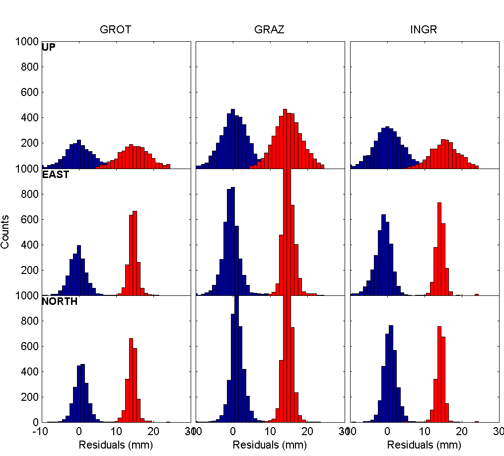
and its estimation reads

(3)

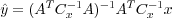
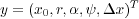
where A is the design matrix, x the observation vector and C_x is the covariance matrix of the observations. Figure 2 shows some examples of site coordinate residuals with respect to the fitted model (1) in the vertical (up) and horizontal (east, north) components.

Figure 2. Coordinate residuals.

[View full size]

Coordinate residuals in the topocentric reference frame (up, east, north) with respect to the linear model: in blue the Gamit and in red the Bernese residuals.