GPS data analysis
Estimating the precise coordinates of a GPS network requires an accurate definition of the reference frame, otherwise the geodetic problem cannot be solved. The normal matrix usually has a rank deficiency equal to the number of parameters needed to define the reference frame datum. The GPS processing scheme subdivides the observations in daily batches and estimates a series of model parameters (troposphere delays, phase ambiguities, Earth Orientation Parameters (EOP) and satellite state vectors (SV)) at convenient frequencies and site positions once a day. Stated in this way, the observation equation is invariant for rigid rotations of the Earth-Satellite system; the normal matrices of the observation equation show a distinct rank deficiency with the same degree of freedom. The rank deficiency is fixed once the orientation of the Earth-Satellite system has been defined or, alternatively, if a number of selected sites and satellites has been forced to the a priori values (ITRF sites and orbits) and the transformation between the reference systems is defined through the EOPs. The classic approach is to fix a number of reference frame parameters in the processing phase or to apply tight constraints to the normal matrix in order to remove the singularity (Biagi and Sansò. 2003, 2004a, 2004b). In the late 1990s and early 2000, a slightly different approach was proposed (Dong et al., 1998; Davies and Blewitt, 2000). The philosophy is to loosely constrain the parameters defining the reference frame (site positions, EOP and SV) leaving all the observations to contribute to the reference frame definition in a consistent way. By not tightly constraining any of the geodetic parameters, we allow the reference frame to be defined in a further step, but on the other hand, some constraints are necessary to prevent the normal matrix from becoming singular. The loose constraints should be chosen weak enough so as not to affect the parameter estimates, but not so weak as to cause significant rounding errors. The main advantage is that no a priori information affects the GPS data processing, thus reducing the risk of possible deformations induced by wrong a priori information.
Both the processing software programs used in this work are able to produce daily loosely constrained solutions that, in principle, are free from any a priori reference frame datum. This means that, since the observations define the reference frame, every daily position is expressed in an unknown reference system, but each reference frame differs day to day in a systematic way dictated by the rank deficiency of the normal equations.
Bernese processing
The GPS data processing is performed by the Bernese software package (Version 5.0; Beutler et al., 2007) forming the double difference of the L1 and L2 phase observations. The GPS orbits and the Earth’s orientation parameters are fixed to the combined IGS (International GNSS Service) products and an a priori error of 10 m is assigned to all site coordinates. The pre-processing phase, used to clean up the raw observations, is carried out in a baseline-by-baseline mode. Independent baselines are defined by the criterion of maximum common observations. The elimination of gross errors, cycle slips and the determination of new ambiguities are computed automatically using the triple-difference combination. The a posteriori normalized residuals of the observations are checked for outliers, too. These observations are marked for the final parameter adjustment. The elevation-dependent phase centre corrections are applied including in the processing the IGS phase centre calibrations (absolute calibrations); moreover, the ocean-loading model FES2004 is adopted (http://www.oso.chalmers.se/~loading/). The troposphere modeling consists of an a priori dry-Niell model improved by the estimation of zenith delay corrections at 1-hour intervals at each site using the wet-Niell mapping function. The ionosphere is not modeled a priori, but removed by applying the ionosphere-free linear combination of L1 and L2. The ambiguity resolution is based on the QIF baseline-wise analysis. The final network solution is solved with back-substituted ambiguities, if integer; otherwise ambiguities are considered as real valued measurement biases.
Gamit processing
To analyze code and phase data with GAMIT software (Version 10.33; Herring et al., 2006), we adopt standard procedures for the analysis of regional networks (e.g., McClusky et al., 2000, Serpelloni et al., 2006) applying loose constraints to the geodetic parameters. We followed a distributed session approach, subdividing the whole dataset into several smaller sub-networks, sharing some common sites. The analysis is performed on a 20-node CPU cluster that makes an efficient use of the distributed session approach.
GAMIT software uses double-differenced phase observations (ionosphere-free linear combinations of the L1 and L2) to generate weighted least-squares solutions for each daily session (Schaffrin and Bock, 1988; Dong and Bock, 1989). An automatic cleaning algorithm (Herring et al., 2006) is applied to post-fit residuals in order to repair cycle slips and to remove outliers. The observation weights vary with elevation angle and are derived individually for each site from the scatter of post-fit residuals obtained in a preliminary GAMIT solution. The effect of solid-earth tides, polar motion and oceanic loading are taken into account according to the IERS/IGS standard 2003 model (McCarthy and Petit, 2004). We apply the ocean-loading model FES2004 and use the IGS absolute antenna phase center table for modeling the effective phase center of the receiver and satellites antennas. We use orbits provided (as g-files) by the Scripps Orbit Permanent Array Center (SOPAC).
Estimated parameters for each daily solution include the 3D Cartesian coordinates for each site, the 6 orbital elements for each satellite, Earth Orientation Parameters (pole position and rate and UT1 rate) and integer phase ambiguities. We also estimate hourly piecewise-linear atmospheric zenith delays at each station to correct the poorly modeled troposphere, and 3 east-west and north-south atmospheric gradients per day to account for azimuth asymmetry; the associated error covariance matrix is also computed and saved in SINEX (Solution Independent EXchange) format.
Imposing the reference frame constraints
The daily GPS solutions are not estimated in a given reference frame since they are computed in a loosely constrained reference frame. Therefore, their coordinates are systematically translated or rotated from day-to-day and their covariance matrices have large errors as a consequence of the loose constraints applied to the a priori parameters (on the order of meters). To express the coordinate-time series in a unique reference frame, associated to their consistent covariances, we have to perform two main transformations. First the loose covariance has to be projected into a well-defined reference frame imposing tight internal constraints (at mm level), and then the coordinates have to be transformed into a given external reference frame - the ITRF2005 catalogue of GPS coordinates and velocities.
In general geodetic problems, the observation equation is invariant for a given symmetry transformation (e.g. the simultaneous translation of the geocentre and the satellite orbits); as a consequence of this invariance, the normal matrix (inverse of the covariance matrix) is singular, and there exist eigenvectors associated with null eigenvalues.
On the contrary, GPS observables (phase double differences) don’t show exact translational symmetry since the satellite orbits are sensitive to the position of the Earth’s center of mass; and weak tracking network and/or poor orbital dynamics require a translational constraint in order to stabilize the solution. Additionally, the GPS observables are not degenerate for scale transformations, but they have errors that may encourage us to constrain the scale. Modeling antenna phase center variations, atmospheric delays and satellite orbits may cause instabilities in the coordinate solutions that can be solved by estimating explicitly translation and scale parameters that can absorb the effects of modeling errors on the estimates. In global GPS networks, the symmetry transformations may have a six-fold degeneracy corresponding to translational and rotational symmetries. Transforming the loosely constrained solution into a well-defined reference frame means fixing the degeneracies (symmetry transformations) and computing the corresponding Helmert transformation (rigid translation, rotation and scaling) to transform the geodetic solution in the given ITRF reference frame.
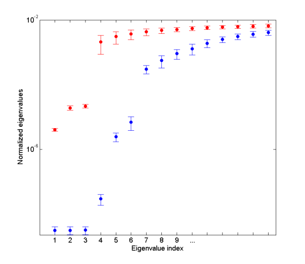
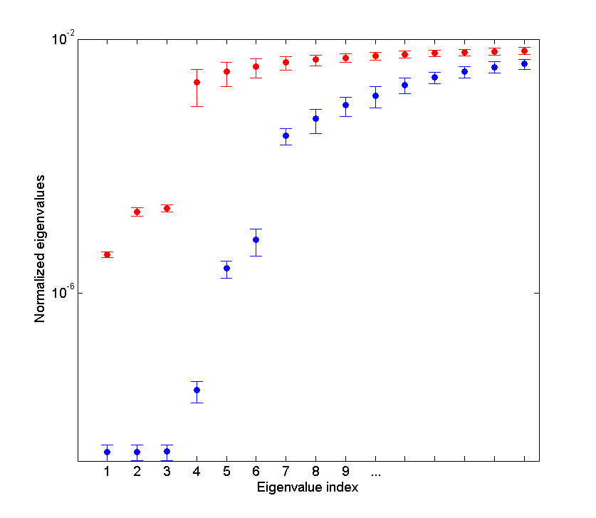
A first guess to establish the proper constraints to be applied is to study the rank deficiency (first eigenvalues) of the normal matrices. Figure 1 shows the first 15 eigenvalues of the daily solutions obtained from the two different analyses. The values represent the average eigenvalues over the entire period and the errorbar represents the scatter from day to day of the corresponding eigenvalue. The main difference arises from the different realizations of loose constraints; namely, in the Bernese approach we fix the EOP and SV to the IGS standard products and apply loosely constraints (10 m) only on coordinates; whereas in the Gamit approach, we loosely constrained the whole reference frame parameters (EOP, SV and coordinates). This reflects directly on the rank deficiency of the normal matrices and, therefore, on the eigenvalues of the daily solutions. The Bernese solutions show three low eigenvalues and often a fourth intermediate eigenvalue. On the other hand, the Gamit solutions show six lower eigenvalues and occasionally a seventh. Therefore, we chose to impose the reference frame through a four-parameter Helmert transformation for the Bernese solutions and a seven-parameter transformation for the Gamit solutions, applying the corresponding constraints to the loose-constrained covariance matrices (see Appendix C of Dong et al., 1998).
Figure 1. First eigenvalues of the Bernese and Gamit normal matrices.
Lowest 15 eigenvalues (average values) of the daily covariance matrices obtained for the Bernese (red) and Gamit (blue) solutions. Each null eigenvalue corresponds to an invariant symmetry (reference frame degeneracy) of the solution. The Bernese and Gamit solutions provide different types of degeneracies.