Experimental setup
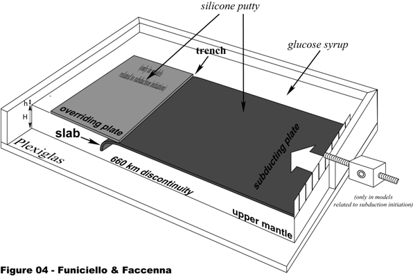
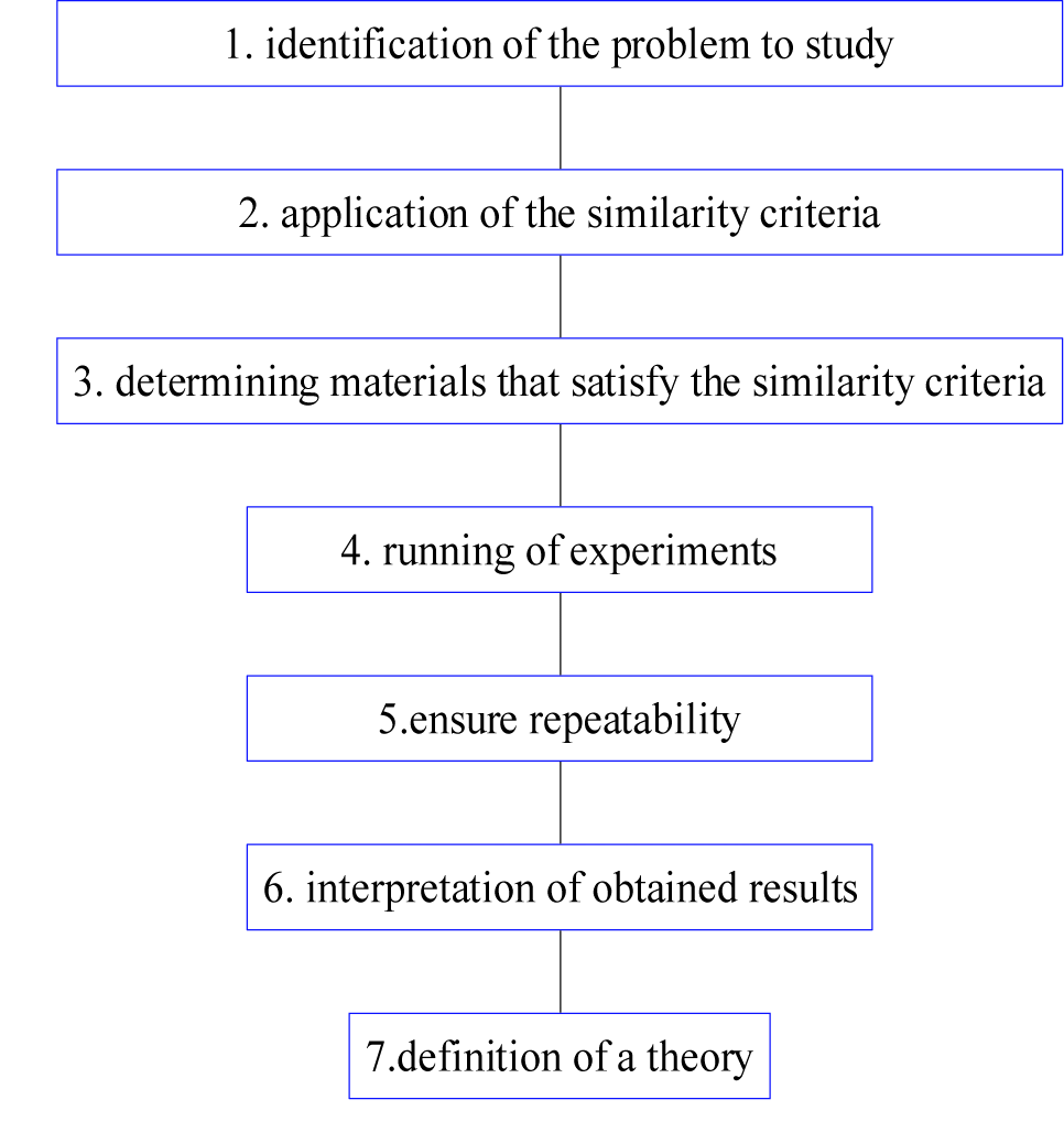
Despite this compact description, the fundamental ingredients needed to describe the Central Mediterranean tectonic framework have been highlighted as follows (STEP 1, Figure 3): a) the presence of slow rates between convergent plates; b) oceanic vs. continental subduction within a laterally heterogeneous continental margin; and c) slab interaction with the 660-km discontinuity.
In the following section, we describe how these observations were converted to input data to design a setup that meaningfully simulates the mechanism governing the slab dynamics, with a specific application to the studied area.
Assumptions
The assumptions underlying the design of our experimental models are listed in the following sections (for more detailed explanations see Faccenna et al., 1999 and Funiciello et al. 2003, Funiciello et al. 2004):
Viscous rheology
The Earth’s profile (i.e., lithosphere and mantle) is simulated using linearly viscous rheologies. A brittle ductile layering is adopted only for models that are finalized with the subduction initiation because we are specifically interested in isolating the role that the brittle and ductile strengths at passive margins play in this framework.
Self-consistent subduction
Justified by the fact that the rate of convergence at the trench has always been very low and the consumption of the lithosphere has been mostly driven by negative buoyancy, that results in trench rollback, slab pull is the only active force within the system. No external kinematic boundary conditions (i.e., plate or trench velocity) are applied. Therefore, the experimental subduction process is a self-consistent response to the dynamic interaction between the slab and the mantle. An exception is represented by models used to study the initiation of subduction, where the incoming plate is slightly pushed by means of a rigid piston that pushes at a constant horizontal velocity with reference to the box boundary.
Convectively neutral mantle
In our experiments flow is generated only by subduction. We neglect thermal convection and the effect of global (Ricard et al. 1991) or local background flow that is not generated by the plate/slab system.
Isothermal models
Experimental limitations lead us to neglect thermal effects during the subduction process. Hence, we assume a constant chemical density contrast throughout the model, and the roles of thermal diffusion and phase changes (Bunge et al. 1997, Lithgow-Bertelloni & Richards 1998, Tetzlaff & Schmeling 2000) are neglected. Consequently, the slab is thought to be in a quasi-adiabatic state. The high subduction velocity (larger than 1 cm/yr in nature) recorded in our models justifies this assumption, ensuring that advection overcomes conduction (Wortel 1982, Bunge et al. 1997).
Lower mantle
It is impossible to reproduce the fundamental role of the endothermic phase change at the transition zone in laboratory. Therefore, because we are interested in exploring the effects of the slab-660 km interaction in the evolution of the Central Mediterranean, the lower mantle is simulated by the increase of viscosity with depth (Davies 1995, Guillou-Frottier et al. 1995, Christensen 1996, Funiciello et al. 2003).
A viscosity increase (by a factor of 10-100) across the 660-km discontinuity has been postulated based on of models of the wavelength of the geoid (e.g., (Hager 1984, Hager & Richards 1989, King & Hager 1994) and the post-glacial rebound (e.g., Mitrovica & Forte 1997). In particular, several models assume that the bottom of the box is analogous to the 660-km discontinuity because this boundary is impermeable for a retreating slab and in the limited timescale of the analyzed process (i.e., <100 Myr; Funiciello et al. 2003).
No overriding plate
Except for models related to subduction initiation, the overriding plate is not modeled to simplify the experimental setting. In these cases, we assume that the fault zone between the subducting and the overriding plates is weak, having the same viscosity as the upper mantle (Tichelaar & Ruff 1993, Zhong & Gurnis 1994, Conrad & Hager 1999). We also assume that the overriding plate passively moves with the retreating trench. This choice, which does not invalidate the general behaviour of the experimental results, appears suitable to simulate the Eurasian plate. However, the rate of the subduction process can be slightly influenced (King & Hager 1990). When we are interested into a more precise kinematic assessment, we introduce a passively moving overriding plate that is positively buoyant with respect to the underlying mantle.
Reference frame
The reference frame for the entire set of models is the box boundary. This frame is considered the experimental analogue to the fixed hot spot reference frame.
Materials
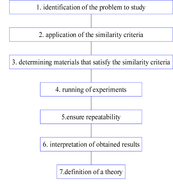
A crucial requirement for experimental models is the ability to scale natural processes to the laboratory enwvironment. Similarity analysis (STEP 2, Figure 3) is the central step in the model design that helps to select the analogue materials, dimensions and rate of deformation. To scale a laboratory model to a natural process, it should be geometrically, kinematically, dynamically and rheologically similar to the prototype (Hubbert 1937, Ramberg 1981). The application of similarity theory starts with the identification of the most relevant physical parameters active into the natural system. Then, each variable (length, velocity, force and material specific parameters) is normalized by means of a dimensionless number. Each set of dimensionless parameters defines a family of equivalent solutions that only differ by a scale factor. The solution, which is characterized by the most relevant scaling, can be used to select materials and design a properly scaled analogue model (STEP 3, Figure 3).
Silicone putty (Rhodrosil Gomme, PBDMS + iron fillers) and glucose syrup/honey were used as analogues of the lithosphere and mantle, respectively. Silicone putty is a visco-elastic material, with purely viscous behavior at low experimental strain rates (Weijermars & Schmeling 1986). Glucose syrup/honey is a transparent, Newtonian, low-viscosity and high-density fluid. For the models used to study the initiation of subduction initiation, a shallow sand mixture layer was added to simulate the brittle behavior of the upper crust. These materials achieved the standard scaling procedure for stresses and were scaled down for length, density and viscosity in a natural gravity field (gmodel = gnature) as described by Weijermars & Schmeling (1986) and Davy & Cobbold (1991).
Table 1. Parameters used in the selected models and in nature.
| PARAMETER | NATURE | MODEL | ||
|---|---|---|---|---|
| g | Gravitational acceleration | m x s-2 | 9.8 | 9.8 |
| Thickness | ||||
| h | Oceanic/continental lithosphere | m | 1 x 10³ | 0.012 |
| H | Upper mantle | 6.6 x 10⁵ | 0.110 | |
| Density | ||||
| ρl | Oceanic lithosphere | kg x m-3 | 3300 | 1482 - 1491 |
| ρcl | Continental lithosphere | 3190 | 1375 | |
| ρum | Upper mantle | 3220 | 1380-1422 | |
| Viscosity | ||||
| ηl | Oceanic lithosphere | Pa x s | 1024 | (1.6-3.6) x 105 (± 5%) |
| ηcl | Continental lithosphere | ≈1024 | 1.8 x 10⁵ (± 5%) | |
| ηum | Upper mantle | 1020- 1021 | 5.5 x 10 - 4.6 x 10²(± 20%) | |
| Time | ||||
| t |
|
3.1 x 10¹³ (1 Myr) | ≈60 | |
The scale factor for length was 1.6·10-7 (1 cm in the experiment corresponds to 60 km). Densities and viscosities were assumed to be constant over the thickness of the individual layers and were considered to be an average of effective values. The scaled density factor between the oceanic lithosphere and the upper mantle ranged from 1.05-1.07 (Molnar & Gray 1979, Cloos 1993). The viscosity ratio between the oceanic slab (ηl) and the upper mantle (ηum) ranged between 102-104. When continental subduction was modeled, the negatively buoyant silicone was laterally joined to a light silicone plate with decreased density over its entire thickness (see Martinod et al. 2005).
Considering the imposed scale ratio for length, gravity, viscosity and density (Table 1) applied to the lithosphere, 1 Myr in nature corresponded to ~1 min in the models for the purely viscous models (i.e., not including models finalized for subduction initiation). Parameters and values for nature and the experimental system are listed in Table 1.
Experimental procedure
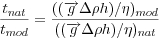
The layered system was arranged in a transparent Plexiglas tank (Figure 4). To limit the lateral box boundary effect, which could alter the results, plates were positioned as far as possible from the box sides (> 11 cm; see Funiciello et al. 2004). Plates were fixed at their trailing edge (“fixed ridge” sensu Kincaid & Olson 1987) to simulate a subduction zone belonging to the stable Africa. Except for the models of the subduction initiation, the subduction process was manually started by forcing the leading edge of the silicone plate downward into the glucose to a depth of 3 cm (corresponding to about 180 km in nature) and with an angle of ~30°.
Each experiment (STEP 4, Figure 3) was monitored using a sequence of digital pictures taken in lateral and top views. Kinematic and geometric parameters (trench motion, plate motion, geometry of the slab at depth, dip of the slab, and surface plate deformation) were then quantified using data analysis tools. Once planned, mantle circulation was analyzed by recording the experiment over its entire duration using two high-velocity, high-resolution, black-and-white progressive scan cameras with two lighted, orthogonal interrogation windows: the x-z plane through the centerline of the tank-slab system and the x-y plane just below the plate at a depth of about 2 cm. In this case, the glucose syrup was preliminary seeded with neutrally buoyant, highly reflecting air micro-bubbles used as passive tracers. These tracers negligibly influence the density and viscosity of the mantle fluid. Movies were stored on a dedicated hard disk and post-processed using the Feature Tracking (FT) image analysis technique (see Funiciello et al. 2006) to retrieve the circulation pattern (i.e., the mantle velocity field, mantle velocity x- and y- components and modulus, the streamlines of mantle circulation, and the mantle linear flux) highlighted by passive tracer particles.
Moreover, the models were repeated several times under the same boundary conditions to ensure repeatability (STEP 5, Figure 3).