Journal of the Virtual Explorer

GES DISC has facilitated pure and applied research by applying cutting-edge information technology to the development of new tools and data services. Giovanni is one such tool that has gained considerable popularity. It continues to evolve in response to science research and application needs (Giovanni 2007a). It is a Web-based interactive data analysis and visualization tool, used primarily for exploring NASA atmospheric and precipitation datasets. With the rapidly increasing volume of archived atmospheric and precipitation data from NASA missions, Giovanni enables users easily to manipulate data and facilitate scientific discovery (Chen, et al. 2008).

The earlier Giovanni Version 2 (G2) (Giovanni 2007a) provides capabilities including area plots, time plots, Hovmöller plots, two parameter inter-comparisons, two parameter plots, temporal correlation maps, etc. All those capabilities can be applied to most NASA atmospheric and precipitation data. Giovanni Version 3 (G3) (Giovanni 2007b) offers many new and more advanced functions, such as vertical data profiling, vertical cross-sections, and zonal averaging. The newest function in G3 is producing multi-instrument vertical plots beneath the A-Train orbit track. G3 provides a useful platform for the utilization of both 2D and 3D geospatial data.

G3 uses a service- and workflow-oriented asynchronous architecture. FTP, HTTP-based scientific data networking software, such as OPeNDAP and GrADS Data Server, are used to enable G3 to access and transfer local and remote scientific data online. Service-oriented architecture requires that all data processing and rendering be implemented through standard Web services. The workflow-oriented management system enables users to easily create, modify, and save their own workflows. This asynchronicity guarantees that more complex processing without the limitation of HTTP time-outs is possible, and that Web services in a process can run in parallel. Finally, G3 is intrinsically extensible, scalable, and easy to work with (Giovanni 2007b).

The A-Train Data Depot is the first instance of the use of G3 for processing and analyzing geospatial data derived from the A-Train satellite constellation (Kempler, et al. 2006). The data can be combined to address scientific problems more comprehensively than is possible with data from any single satellite dataset (Vicente, et al. 2006). At present, vertical data from three of the seven satellites in the A-train – CloudSat, CALIPSO, and Aqua – are processed using G3 and integrated together in Google Earth.

Users can launch a G3 web-based graphical user interface to input spatial and temporal criteria to produce a curtain plot image. The interface lists all available parameters that users can customize to their specific requirements. When the user selects the input parameters from the interface, the user interface software creates an XML representation of the inputs, and initiates execution of the appropriate workflow. For the asynchronous case, when the workflow processing is complete, the URL of the resultant product (usually an image) is available. When the processing is fast and appears to be synchronous, the result will be directly returned to the user, usually via the Web browser (Berrick, et al. 2006).

The following geospatial vertical data are processed in G3 to be rendered into the curtain plot, to reveal different physical phenomena with different physical parameters:

Figure 4. Image curtain of vertical data from CALIPSO in G3

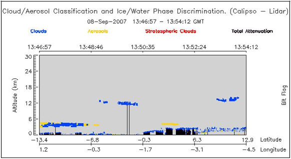
A Perl script automatically acquires the vertical data image curtain. First, the script produces the requested parameters file in XML format for the temporal range selected and inputted by the user. In the parameters file, the temporal range and the specific satellite orbit model are used to calculate the spatial range. Other parameters depend on the relevant physical variable, e.g.. Radar Reflectivity or Received Echo Powers. Second, the parameters file is used to invoke a workflow from G3 to transparently access the vertical data. Finally, a series of procedures such as sub-setting, extracting, scaling, stitching, and plotting are used to process the data to output the curtain plot image (Chen, et al. 2008). Figure 4 shows a curtain plot for Cloud/Aerosol Classification and Ice/Water Phase Discrimination from CALIPSO in A-Train system

Google Inc. provides a 3D tool named SketchUp (Google 2007b). SketchUp is used to save a Collada model, which defines a 3D model that can be imported into Google Earth for visualization. Collada is for establishing an open, standard, XML-based Digital Asset schema for interactive 3D applications (Barnes 2006). Here, its real 3D features are used to represent geospatial vertical data

Figure 5. Rendering the orbit curtain from vertical data

Figure 5 illustrates the rendering procedure of an orbit curtain for vertical data in Google Earth. The image curtain output is produced using G3 and chopped into small size image slices. The Collada model’s template is created via SketchUp. The image slices are applied to the model template to form a series of Collada models. In order to assemble those 3D models accurately along the satellite orbit track in Google Earth, the coordinate system of SketchUp (x, y, z) must be mapped to that of Google Earth (Longitude, Latitude, Altitude). The model template has an x value, z value, and approximately (but not exactly) zero y value, which makes the model 3D, but it looks like a thin curtain. The model’s x-z plane is textured with the transparent vertical data image slice. The 3D model can be finally exported out as a KML Zipped (KMZ) file, which is supported in Google Earth. The KMZ file zips all related files required for visualizing this model in Google Earth. It usually includes, at the minimum, a KML file, image file(s), model file(s), and a texture file. The KML file determines the spatial coordinates, the level of zooming out, and the number of degrees of rotation needed to accurately visualize each model along the satellite orbit track to form the orbit curtain in Google Earth. The Texture file determines the images used as texture for models.

The spatial coordinates for each model are calculated from the satellite orbit model and the orbit time in the form of year, month, day, hour, minute, and second (Durden, et al. 2004). Considering the rendering speed and accuracy of the orbit curtain in Google Earth, 10 seconds is selected as the minimum temporal range whose corresponding spatial range is represented by each model. The corresponding spatial range (about 67.7km) serves as a reference for determining the x value of the Collada model. The zoom scale in the x and z directions, is calculated from the x and z sizes, respectively, of the model and the real size represented by the model in Google Earth. The rotation degree of the model is derived from the coordinates of two endpoints of the orbit represented by the model. The detailed calculation formulas are available in Chen, et al. (2008). Table 3 is part of the KML codes for one image slice on the orbit track. It shows geospatial coordinates, rotation degree, and the scale of zoom-out for the 3D model.

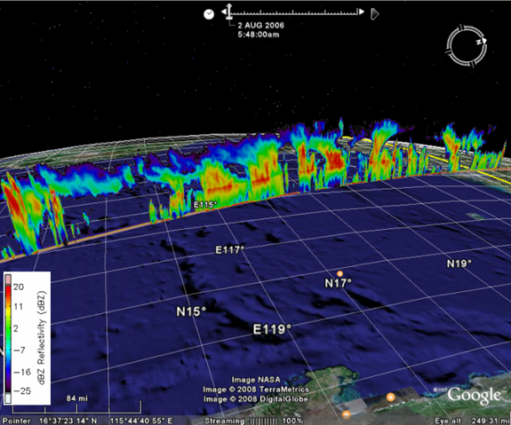
This solution accurately places vertical image slices along the orbit track in Google Earth. Figure 6 shows part of the orbit curtain for cloud reflectivity (dBZ) from the CloudSat satellite. This vertical data orbit curtain function has been closely integrated into the Giovanni A-Train operation system. Users can directly download the KMZ file after they view the image curtain in their Web browser and open it as a curtain plot to overlay with any other scientific products in Google Earth.

Figure 6. The orbit curtain of CloudSat (radar reflectivity - dBZ) in Google Earth