In FLAC modeling, the solid body ("sample") is divided into a finite difference mesh composed of quadrilateral elements, called zones. In FLAC's actual calculation, a zone is subdivided into 2 sets of triangles (Figure 4). A quadrilateral zone may be deformed in any fashion, subject to (1) the area of the quadrilateral being positive, and (2) each member of at least one pair of triangles being >20% of the total quadrilateral area. If either criterion is violated, FLAC issues an error message of "bad geometry" and the modeling cannot proceed further. This limits the amount of bulk strain that can be reached for some numerical runs.
The geometry of the model setup is schematically shown in Figure 5. A homogeneous Mohr-Coulomb body of 100m by 100m containing a horizontal ubiquitous joint (anisotropy plane) is subjected to shortening parallel to the anisotropy. A displacement boundary condition is applied and the specimen is confined under a pressure of 500MPa throughout deformation. The lateral boundaries are frictionless (Figure 5). A grid size of 1 meter by 1 meter is used (that is the sample has in total 10,000 equal sized zones). We have tested possible effects of grid size on modeling results by reducing the zone size to 0.5m by 0.5m for some numerical runs, and the results are quantitatively identical to those with a grid size of 1m by 1m. All results presented below are for 1m by 1m grid size situations.
Figure 4. FLAC numerical modeling
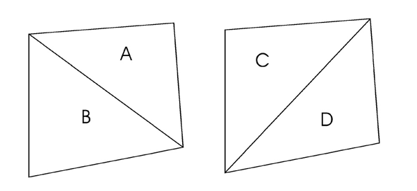
In FLAC numerical modeling the sample is divided into a finite difference mesh of quadrilateral elements called zones in which the deformation is homogeneous. Each zone is subdivided into 2 pairs of triangles (A and B, C and D). The distortion of a zone must be within certain limits so that the zone does not run into "bad geometry". See text for more discussion.
Figure 5. Geometric setup of the numerical modeling
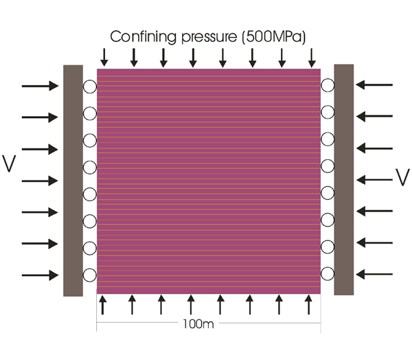
Geometric setup of the numerical modeling. See text for details.
The following material properties for the Mohr-Coulomb solid compiled from the rock type shale of Carmichael (1989) are used: density 2500kg/m3, bulk modulus 2.81x10⁴ MPa, shear modulus 1.69x10⁴ MPa, cohesion (C) 3.0MPa, tensile strength (T) 1.5 MPa, friction angle (f) 30°, and dilation angle (for definition see Ord 1991) 4°. Mechanical properties of the ubiquitous joint ("foliation") are: cohesion (Cj) 7.5x10⁻³ MPa, tensile strength (Tj) 4x10⁻³ MPa. The friction angle (fj) for a specific modeling run is calculated according to equation 6 for a given m value. An incremental displacement of 1mm per step is used, which means that for every 1000 steps, 1% of bulk shortening is achieved. A specimen is shortened to as high a strain as possible, until a zone develops "bad geometry".
At the end of a model run, the grid coordinates of points whose history is of interest are identified. The model is then rerun with the histories of marked points recorded using FISH programs developed at Maryland.