Figs. Figure 6, Figure 7, Figure 8, and Figure 9 show progressive evolution of the specimen as deformation advances for four numerical experiments identical in all respects except the m values. The banding in these figures serves as passive markers parallel to the anisotropy. They do not have any mechanical significance. The following observations are readily made from these figures.
When m = 2 (Figure 6), the modeling reaches a maximum bulk shortening of 11%. Conjugate kink-bands develop. They are simple kink-bands. α ≍ 40° when the kink-bands are clearly defined at 8% shortening. Kink bands rotate slightly as strain increases (α ≍ 42° at 11% of strain). KBB's migration is clearly indicated by widening of kink-bands as deformation advances (Figure 6a and b) and by the concentration of incremental strain at KBB's. As kink-bands widen, b increases from 0 to being close to a. Foliation within the KBD remains planar. Outside the kink-bands, the foliation remains planar and the strain is low (~4%, Figure 10, see below). Figure 6c is a contour map of the instantaneous shear-strain increment per step, the second invariant of the incremental strain tensor, at the instant the bulk strain is 10%. It shows that as b approaches a, active deformation occurs only at the migrating kink-band boundaries; the interior of the band is practically inactive. Both bounding boundaries of a kink-band may be migrating (solid white arrows in Figure 6c), or only one boundary is (open white arrows in Figure 6c).
Figure 6. Modeling results for m=2
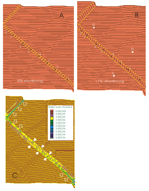
Modeling results for m = 2. (A) Conjugate kink-bands occur as strain localization bands. (B) Kink-bands widen by migration of kink-band boundaries. (C) The incremental shear strain of at the state when bulk shortening is 10%. High-shear incremental shear strains are at both kink-band boundaries (solid white arrows), or one kink-band boundary only (open white arrows). Yellow lines are the orientation of ubiquitous joints. Numbered and lettered gridpoints are those whose stress and strain histories are recorded (Fig. 10).
Figure 7. Modeling results for m=5
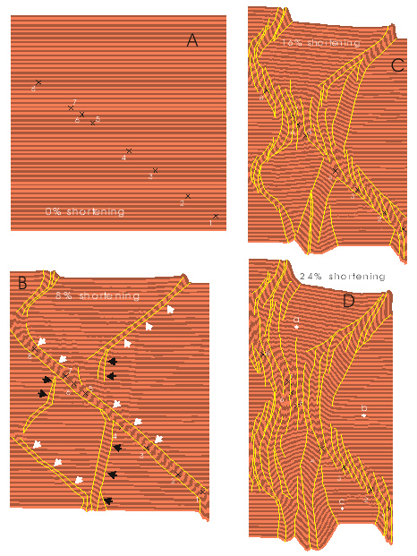
Modeling results for m=5. (A) The undeformed state. (B) At 8% of shortening, both conjugate kink-bands (white arrows) and high-angle kink-bands are initiated as strain localization zones. The former are composite kink-bands. (C) Migration of kink-bands is clear. Within conjugate kink-bands, kinks have their axial planes in an en echelon array. High-angle bands develop into kinks. (D) Kink-bands continue to widen and kinks tighten as bulk shortening advances.
When m=5 (Figure 07), at a low value of bulk shortening (8%), conjugate kink-bands (white arrows in Figure 7b), as well as kink-bands at higher angle to the foliation (high-angle bands hereafter, black arrows in Figure 7b) develop. Unlike m=2 case, the conjugate kink-bands are composite bands (with further kinks in them). As bulk shortening further increases (16% and 24%), all kink-bands widen, and more new high-angle bands emerge. Earlier high-angle bands evolve into kink folds or box-like folds (bottom part in Figure 7c and d). Thus the high-angle bands are initial stages of kink and box-type folds. Kinks within conjugate kink-bands have their axial planes arranged en echelon within their hosting bands, consistent with the sense of shear of the hosting kink-bands. As shortening increases, all bands rotate toward higher angles with respect to the shortening direction. Merging of conjugate kink-bands is observed only in the vicinity of the intersection of two conjugate bands.
As m is further increased (m=10, Figure 08), strain-localization-type conjugate kink-bands observed in Figures 6 and 7 are absent. Only high-angle bands kinks with axial planes close to normal to the shortening direction, develop. At low strains (e.g., <16% shortening, Figure 8a and b), one can identify a broad zone of concentrated kinks in the orientation of conjugate kink-bands Figure 8a. When m=20 (Figure 9), the deformation is achieved completely by pervasive kinking throughout the specimen.
Figure 8. Modeling results for m=10
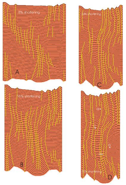
Strain-localization type bands do not develop. Only kinking occurs, but kinks concentrate in a broad zone in the orientation of conjugate kink-bands at low strains (A). As strain increases (B, C, and D) this zone is obscured and overall geometry resembles symmetric kinks.
Figure 9. Modeling results for m=20
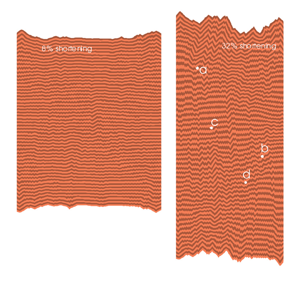
The mode of deformation is entirely kinking in the whole volume of the specimen.
In order to determine the history of kink-band development and examine whether kink-bands develop from a point source, we select a number of material points inside and outside of a kink-band from the final configuration of modeling runs (numbered and lettered grid points in Figures 6, 7, 8, and 9), identify their grid coordinates, and rerun the modeling to record the stress and finite strain histories of these points. A FISH program 'strain_his" was developed to retrieve the history of Rf = (1 + e1) / (1 + e3) where e1 and e3 are respectively the two principal elongations) for selected points.
Figures 10 and 11 are plots of the accumulation of finite strains for m=2 and m=5 cases respectively. Points 1 through 8 are inside a kink-band and points a, b, and c outside of the kink-band (Figures 6, 7). Outside the kink-band domain, finite strain increases to a low value and remains nearly constant thereafter (Figure 10b and Figure 11b). The maximum strain ratio outside kink-bands is around 1.1, except for point a in the m=5 case (Figure 11b), for which the higher strain is interpreted as being due to development of local kinking. Rf = 1.1 corresponds to principal elongation values of e1=4.4% and e3=-4.2%, which are close to the bulk shortening value at the time the kink-band starts to develop (Figure 10a and Figure 11a). This implies that for m=2 and m=5 cases, once kink-bands start to develop, strain remains approximately constant outside kink-bands. That is, deformation is nearly entirely localized into kink-bands.
Figure 10. History of finite strain accumulation (m=2)
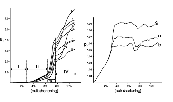
History of finite strain accumulation for gridpoints inside (1 through 8) and outside (a, b, and c) a kink-band for m=2 case. Strain outside the kink-band remains approximately the same after kink-bands are initiated. Strain inside kink-bands increases rapidly after kink-bands are initiated. See text for further discussion.
Figure 11. History of finite strain accumulation (m=5)
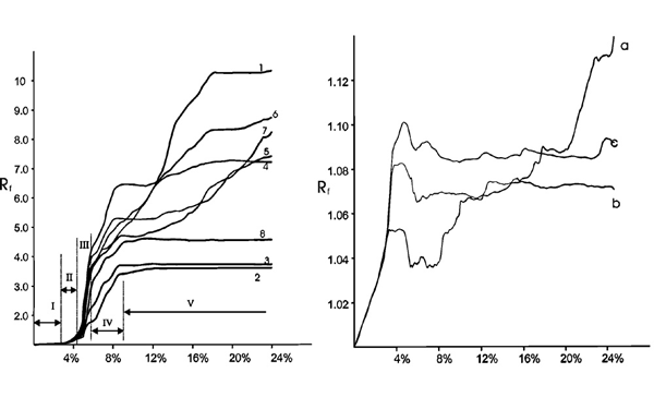
History of finite strain accumulation for gridpoints inside (1 through 8) and outside (a, b, and c) a kink-band for m=5 case. Following initiation of kink-bands, strain outside the kink-band remains approximately the same but increases rapidly inside the band until the kink-band "locks" (stage V). See text for further discussion.
We describe the accumulation of finite strain inside the KBD in terms of 5 stages (Figs. 10A and 11A). Stage I evidently corresponds to homogeneous elastic deformation throughout the sample. In stage II finite strain increases at an increased rate, corresponding to the initiation of kink-bands. This stage is followed by stage III, an accelerated increase in the rate of finite strain accumulation, marking the instability associated with kink-band formation. All marked grid points inside the kink-band follow similar strain increase path, suggesting that strain localization rather than kinematic growth from a line or point source is responsible for the onset of kink-bands. Following stage III, the rate of strain increase is reduced and, if the sample can be deformed further without running into "bad geometry" (m=5 case), strains at many points may reach a maximum value and then cease to increase (stage V, Figure 11a). We interpret this as indicating the "lock-up" of kink-bands.
In terms of stress history (Figure 12), for both m=2 and m=5 cases, the initiation of kink-bands is marked by a drop in axial stress followed by a further accelerated drop in axial stress. The initial stress drop is interpreted as being due to yielding of the Mohr-Coulomb solid and the accelerated drop is interpreted as being due to yielding along the anisotropy and localization of strain into kink-bands. Following that, the axial stress climbs up to a level close to the initial yielding (peak) stress for the m=2 case. Further evolution of the stress is unclear for them=2 case because the modeling was terminated at 11% bulk shortening due to "bad geometry". We speculate that the stress most likely will exhibit cyclic fluctuations as schematically shown in m=2 case of Figure 13, as new kink-bands develop continually. For the m=5 case (Figure 12), after the stress drop associated with kink-band instability, the axial stress climbs up to a level noticeably below the initial yielding stress and then fluctuates at this level. We interpret this as being associated with kinking outside kink-bands as well as broadening of KBD's (Figure 6, Figure 13 m=5 case).
Figure 12. History of axial (horizontal normal) stress
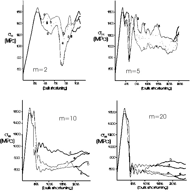
History of axial (horizontal normal) stress for marked gridpoints for the four numerical experiments of m=2, 5, 10, and 20. See text for discussion.
Figure 13. Simplified and schematic stress-strain
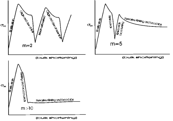
Simplified and schematic stress-strain curves for low (m=2), intermediate (m=5), and high (m>10) degree of anisotropy. See text for discussion.
As the material becomes more anisotropic (the m=10 and 20 cases), the stress history is different in two respects (Figure 12, m=10 and 20 cases). First, the separation between the initial drop in axial stress, interpreted as marking the yield of the Mohr-Coulomb solid, and the drop interpreted as yielding of the foliation, is strongly subdued (for the m=10 case) or barely visible (for the m=20 case). This suggests a rapid transition from yielding of the solid to yielding of the foliation. Second, the climb-up of stress following yielding is almost absent. The axial stress fluctuates at a very low level (close to the confining pressure for the m=20 case), corresponding to pervasive kinking. This indicates that, if a material is highly anisotropic, it cannot support high differential stress once the foliation is kinked (Figure 13, m> 10 case).