In order to model the dissolution of stressed elastic solids we use a hybrid approach. The dissolution rate is calculated with a first order kinetic rate law from Transition State Theory. It depends on the local Gibbs chemical potential of the solid-liquid interface. The discrete element model is used to calculate the stress and elastic energy distribution in the crystal after it is being loaded. The surface energy is also determined from the elastic model and depends on the number of springs that particles have towards boundaries, which is a function of the larger scale surface curvature. Most parts of the simulations are performed with the numerical model "ELLE" [Jessell et al. 2001], which we have expanded by the discrete element code "MIKE".
In order to treat the dissolution of the stressed solid we relate the change in chemical potential as defined in equation 1, which is due to a change in elastic or surface energy, which are contained within the Helmholtz free energy (Δψs), to the change in local equilibrium concentration (ΔC) of dissolved matter in the fluid by the relation:
where R is the universal gas constant and T the temperature [Koehn et al. 2003]. The dissolution rate of the local surface can then be calculated using a linear rate law following Transition State Theory [Lasaga 1998]:
where D is the velocity of dissolution perpendicular to a unit surface and kr a rate constant depending on temperature and activation energy. We assume that the fluid volume is very large so that the concentration of dissolved matter in the fluid does not change [Koehn et al. 2003] and the dissolution rate depends only on the change in equilibrium concentration of the fluid from a system with a non-stressed crystal to a stressed crystal. This assumption is valid for the case of the den Brok and Morel (2001) experiment where the system was constantly slightly under-saturated and the fluid volume very large.
Figure 1. Two-dimensional networks
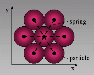
In the two-dimensional lattice that is used for the simulations particles are arranged in a triangular network. Each particle (except for boundaries) is initially connected with six springs to six possible neighbors.
The elastic crystal in a simulation is modeled using a discrete element approach. In this model circular particles are arranged in a triangular lattice and connected by linear springs with each other (Figure 1). In a triangular configuration each particle is connected with six possible neighbors. The force on a particle from a spring is proportional to the actual length of the spring minus an equilibrium length times a spring constant so that compressive stresses in the model are by definition negative (Figure 2). The equilibrium configuration of particles and the stress field in the elastic crystal are found by a standard over-relaxation method [Allen 1954]. Particles are moved until forces that act on a single particle cancel out and an equilibrium configuration for the lattice is found. It has been shown that the triangular lattice in two-dimensions reproduces linear elasticity on a large scale [Flekkøy et al. 2002]. Therefore it can be used to model systems that behave linear elastic.
However, the model can describe the behavior of the solid beyond linear elasticity by introducing the possibility to break springs. Springs are broken once they reach a breaking-threshold defined by a maximum local tensile stress that one spring can sustain. If the tensile stress on the spring is larger than the threshold it breaks and is removed from the lattice so that the previously connected neighbors loose their cohesion. All particles have repulsive forces between each other even if springs are removed and the particles are not really connected. Single springs can never break under pure compression. It has been found that fractures that develop in the model are very similar to fractures found in experiments [Walmann et al. 1996; Malthe-Sørenssen et al. 1998]. In order to add noise to the system to minimize lattice effects a pseudo random distribution of breaking thresholds and spring strengths can be applied to the model [Koehn and Arnold 2003, this volume].
Figure 2. Particles under compression
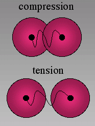
Under compression particles are pushed into each other, under tension they move away from each other. Springs can only break under tension. Particles are repulsive so that they always have a compressive force between them.
The discrete element model has three possible boundary conditions that were used in the presented simulations: Lattice boundaries, internal boundaries and three-dimensional boundaries due to deformation estimates.
Two different lattice boundaries exist in the model (Figure 3). These consist either of 1. a row of particles (particle walls) along the boundary of the lattice or 2. elastic walls along the rims of the deformation box. 1. Boundary particles of particle walls are defined to be part of the lattice boundary, which means that they are moved during a deformation step and then remain stationary during the relaxation. Boundary particle springs cannot break. 2. Elastic walls are walls that act with a compressive force on the particles where the force is proportional to the distance that particles are pushed into the wall. Depending on the elastic constants of walls relative to constants of normal particles walls are either stiff (higher constant) or soft (lower constant). Elastic walls apply no friction or tension on boundaries of the model in contrast to boundary particles.
Figure 3. External boundaries
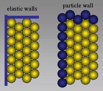
Two possible external boundaries are applied in the simulations. The picture on the left illustrates elastic walls. Particles have repulsive forces on walls so that the force on a particle from a wall is proportional to the distance that the particle is pushed into the wall. Particle walls are rows of particles on the boundary that are moved only during a deformation step and stationary during relaxation.
Internal boundaries of the model are grain or hole boundaries. Single grains are made up of a cluster of particles that lie within a specified area (Figure 4). Particles on the rim of the grain are defined as being part of a grain boundary. Springs that connect two grains and cross a boundary can have different spring constants and different breaking strengths than springs that lie within grains. Particles that are on the rim of grains or holes can have surface energies and can react with for example fluid in a hole. The surface energy depends on the absolute size of a particle and on the number of springs that are part of a boundary. The number of boundary springs then defines the surface curvature.
Figure 4. Clusters of particles
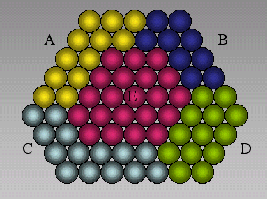
Grains A to E are defined by clusters of particles. Springs between particles of different grains can have different properties than springs within grains.
We apply deformation estimates. If a wall of the lattice is moved inwards to stress a crystal all particles are moved according to that deformation assuming that the material is homogeneous. The relaxation starts after this average is taken. Such a deformation estimate will remove boundary effects from the walls. It will also have the effect that the model is quasi three-dimensional so that even if the model has no cohesion in two dimensions (for example a through-going hole or crack in the center) it has a cohesion in three-dimensions. Instead of applying deformation estimates one can also attach springs to particles in the third dimension and attach these to a homogeneously deforming sheet [Malthe-Sørenssen et al. 1998].
The discrete element code and the dissolution routines are coupled in two ways. First of all the elastic energy and surface energy of internal boundary particles in the discrete code are used as input for the dissolution routines to calculate a dissolution velocity (or reaction velocity) of a unit surface. In a second step this dissolution rate is then used to calculate a probability of how often a particle on the boundary will dissolve in a given time step according to
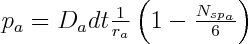
where Da is the dissolution rate for particle a from equation 3, ra is the radius of particle a and Nspa the number of springs that are still attached to the particle. The last term on the right hand side of equation 4 is representative of the particles circumference that is in contact with the fluid. The 1/r term represents the size of the particle. For example, a smaller particle has a higher probability to dissolve than a large particle. A particle with 4 open springs has a higher probability to dissolve than a particle with 2 open springs because its reactive "surface" that is in contact with the fluid is larger. Particles that shrink completely within a given time step are removed from the discrete model. All other particles shrink in area depending on their probability to dissolve. The elastic model will not be influenced by the reduction of a particle's area until the particle has completely dissolved and is removed from the elastic lattice. In order to add noise to the system a pseudo random distribution can be applied to the area of the particles. This will only affect dissolution and not the effective size of the particle in the elastic model.