How To Measure Dihedral Angles
Early work on dihedral angles was done primarily on metals (Smith, 1964) and sulfides (Stanton and Gorman, 1968): these are opaque and so the first measurement techniques developed were appropriate for polished sections. The apparent dihedral angle measured on a 2-D section through a polycrystalline material depends on the relative orientation of the grain boundaries and the sample surface, being either higher or lower than the true value. Smith (1948) demonstrated that in a sample with randomly oriented grain boundaries and a single value of true dihedral angle the mode of a theoretical distribution of apparent angles has the same value as the true dihedral angle. However, the mode is a difficult parameter to constrain accurately as it requires a large population of measured angles: ~200 measurements are required to obtain a value for the mode which lies within 5˚ of the true angle (Harker and Parker, 1945). An easier measure to constrain is the median, and the median of a theoretical distribution of apparent angles is always within 1˚ of the true value. Riegger and Van Vlack (1960) showed that only ~25 measurements to achieve a similar degree of accuracy to Harker and Parker (1945).
Many studies of geological materials rely on observation of polished opaque fragments (e.g. experimental run charges) and therefore are reliant on interpretation of apparent angles. However, as first pointed out by Stickels and Hücke (1964), many observed distributions depart from those predicted for equilibrated single-valued aggregates. The departure may be due to errors in measurement or the effects of preferred alignment of non-equant grains via a variation of apparent particle size. For most geological materials it is likely that the bulk of the departure is caused by the presence of a range of true angles, due either to incomplete textural equilibration or crystalline anisotropy (Laporte and Provost, 2000; Leibl et al., 2007). Extracting the range of true angles from a set of measurements from a 2-D section is not straightforward (Riegger and Van Vlack, 1960; Stickels and Hücke, 1964; Jurewicz and Jurewicz, 1986; Vernon, 1997; Laporte and Provost, 2000).
As pointed out by Vernon (1997) the interpretational problems associated with measurements of apparent angles can be avoided completely for translucent samples. The range of true angles in a petrological thin-section can be constrained directly using a universal stage mounted on an optical microscope (see the accessible review by Kile (2009)). This instrument permits the rotation of grain boundaries into alignment with the line of sight, thus permitting the measurement of the true dihedral angle. True angles can be also measured using transmission electron microscopy (Cmíral et al., 1998). Early work on dihedral angles in geological materials used the universal stage (e.g. Voll, 1960; Vernon, 1968) but it subsequently fell into general disuse, perhaps because it is no longer introduced to undergraduates, having become obsolete for many of its original purposes.
Use of the universal stage requires a petrological microscope with a sufficiently large distance between the objectives and the planar rotating stage (most microscopes dating from 1970 or earlier will suffice) together with a long working distance objective (such as those used for heating stages for fluid inclusion work). The minimum magnification for dihedral angle work is about x30 (I use the Leitz UM32 objective; no longer in production but obtainable from collectors and traders in microscope equipment).
Universal stage measurement of dihedral angles can be learnt quickly. The angle to be measured (generally in plane–polarised light) is located at the cross-hairs and the section is rotated (using trial and error) until all three grain boundaries in the immediate vicinity of the junction are sharply defined (and thus oriented parallel to the direction of view). It is important that the angle is measured right at the junction itself, and for curved boundaries it is necessary to measure the angle between the tangents to the boundary (Figure 1d) – this takes practice but is otherwise straightforward. A further consideration is that many grain boundaries may be facetted in the immediate vicinity of the junction and care must be taken to measure the angle at the junction itself (Kruhl, 2001). The analyzer can be used to provide a check that the boundaries are truly parallel to the direction of view: inclined boundaries in relatively highly birefringent materials will have variable birefringence or interference fringes. Measurement of the angle is then a matter of using the gradations on the rotating stage to read off the angle between the two boundaries of interest.
Measurement errors
There are several possible sources of error in determining the dihedral angle population. The first, relevant to measurement of both apparent angles in 2-D and true angles in 3-D, is a simple measurement bias, with undue emphasis given to angles in a particular size range. The universal stage provides a useful check on this possibility, since the observer does not generally have much idea how large the angle is until some effort has been expended in orienting the junction correctly. However, a major source of possible sampling error for very large angles arises when the A-A grain boundary (for the angle at A-A-B junctions) is not clearly visible. Such high angles may be easily overlooked as they will appear to be part of a single A-B junction: this problem typically occurs when measuring augite-plagioclase-plagioclase angles in plane polarized light. A simple way to avoid this is to insert the analyzer when searching for angles to measure, making it obvious where the plagioclase-plagioclase grain boundaries meet a grain of another phase.
Another source of error is that associated with an individual measurement. Each researcher needs to determine his or her own margin of error, perhaps by measuring the same angle many times. It is typically of the order of a few degrees (e.g. Gleason et al., 1999).
The final source of error is more complex. Because we don’t know the distribution function of the underlying (parent) population that is being sampled, it is not straightforward to work out the error on the median or standard deviation of a population of measured angles. Stickels and Hücke (1964) developed a non-parametric method, based on the assumption that the population has a continuous distribution function of some unknown form, to establish a confidence interval for the median angle of a population independent of its actual distribution. They present the confidence intervals as a function of different sample sizes (reproduced here as Table 1). For example, for a sample of 100 measurements, listed in order of their magnitude, there is only one chance in twenty that the median value will not lie between the values of the 40th and 60th measurements.
Table 1. Confidence interval for population median for samples of various sizes
| Sample size | 90% confidence interval | 95% confidence interval | 99% confidence interval |
|---|---|---|---|
| The confidence interval for the median of a population sampled by varying numbers of individual measurements. From Stickels and Hücke (1964). | |||
| 25 | 9 to 17 | 8 to 18 | 6 to 20 |
| 50 | 19 to 32 | 18 to 33 | 16 to 35 |
| 75 | 30 to 45 | 29 to 46 | 26 to 50 |
| 100 | 42 to 58 | 40 to 60 | 37 to 63 |
| 250 | 112 to 138 | 110 to 140 | 105 to 145 |
| 500 | 232 to 268 | 228 to 272 | 221 to 279 |
| 1000 | 474 to 526 | 469 to 531 | 459 to 541 |
To illustrate the errors associated with dihedral angle measurements a suite was chosen of nine samples with very different dihedral angle populations (Figure 2a and Table 2, with the full data set provided in Table 3.) Click to download Table 3. For each rock, a large number of measurements were made of the true dihedral angle. Several thin sections were used for rocks in which suitable three-grain junctions were rare. The standard deviations of the parent populations vary from 10˚ to 25˚, with median values between 60˚ and 114˚. There is a negative correlation between the median and standard deviation (c.f. Holness et al., 2005a). The error on the median was determined using the method of Stickels and Hücke (1964), and the 95% confidence interval is presented in Table 1. The error associated with each median value increases with the spread of the populations.
Figure 2. An analysis of errors associated with the standard deviation and the median dihedral angle
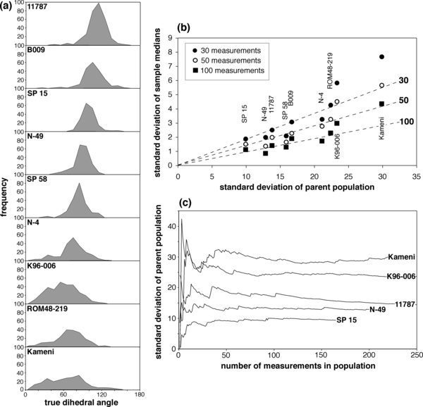
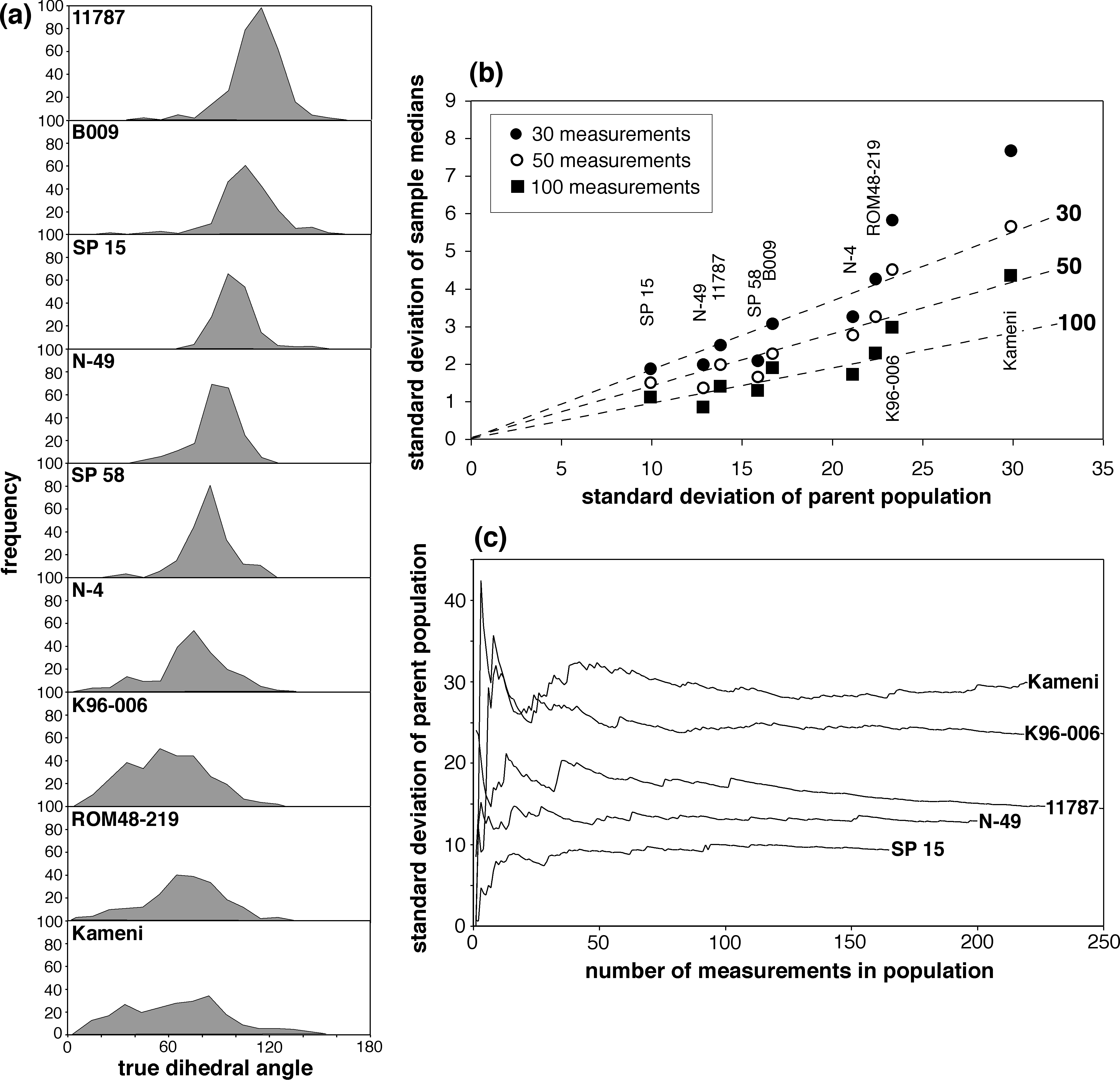
(a) frequency plots of true dihedral angles measured in the series of rocks detailed in Table 2. (b) The standard deviation of the median value of a small population taken from the larger populations shown in (a), plotted as a function of the standard deviation of the parent population. The dashed lines are the standard deviations of the median calculated assuming the parent population has a normal distribution labeled according to the number of measurements taken from the parent. (c) The standard deviation of a population as a function of the increasing number of measurements for a representative subset of the nine rocks shown in (a) and (b).
Table 2. Errors associated with dihedral angle measurements
| Sample | Phases | n | median | s.d. | Description | Locality | Reference |
|---|---|---|---|---|---|---|---|
| SP 15 | augite-plag-plag | 166 | 99° ± 1° | 10.0° | gabbro | Skaergaard Marginal Border Series | Kramer Ø |
| N-49 | augite-plag-plag | 201 | 90° ± 1° | 12.9° | gabbro | Rum Eastern Layered Intrusion, Unit 10 allivalite | Sides (2008) |
| 11787 | augite-plag-plag | 300 | 114° ± 1° | 13.8° | granulite | Peruga, South India (Harker Collection | Cambridge) |
| SP 58 | augite-plag-plag | 200 | 84° ± 1° | 15.9° | gabbro | Skaergaard Marginal Border Series | Kramer Ø |
| B009 | augite-plag-plag | 200 | 106° ± 2° | 16.7° | gabbro | Rum Eastern Layered Intrusion, Unit 9 allivalite | Holness et al. (2007b) |
| N-4 | augite-plag-plag | 200 | 74° ± 2° | 21.2° | troctolite | Rum Eastern Layered Intrusion, Unit 10 allivalite | Sides (2008) |
| ROM48-219 | augite-plag-plag | 200 | 71° ± 3° | 22.4° | dolerite | Traigh Bhan na Sgurra sill, Ross of Mull. | Holness & Humphreys (2003) |
| K96-006 | glass-amph-amph | 300 | 60° ± 3° | 23.3° | enclave | Kula Volcanic Province, Western Turkey | Holness & Bunbury (2006) |
| Kameni | glass-plag-plag | 230 | 66° ± 5° | 29.9° | enclave | Kameni Islands, Santorini, Greece | Martin et al. (2006) |
| 70424 A | augite-plag-plag | 100 | 98° ± 1.5° | 8.9° | gabbro | Stillwater Intrusion, Montana. ⊥ foliation | From the Harker Collection |
| 70424 B | augite-plag-plag | 100 | 99° ± 2° | 9.1° | gabbro | Stillwater Intrusion, Montana. ⊥ foliation | |
| 70424 C | augite-plag-plag | 97 | 98° ± 1.5° | 9.0° | gabbro | Stillwater Intrusion, Montana. // foliation |
Using these large measurement populations we can simulate the process of taking a limited sample population from an unknown parent population and approximate the effects of sample size. 200 random sample populations of 30, 50 and 100 angles were chosen from these parent populations (i.e. 600 randomly chosen sample populations for each rock). The median values for each of the 600 randomly chosen sample populations vary about the median of the parent population. The standard deviation of this variation provides a measure of the accuracy of the median values for the sample populations and, as expected, the median values show less variability within the larger sample populations. The standard deviation, 1σ, of these median values is shown as a function of sample size and the standard deviation of the parent population in Figure 2b. For comparison the standard deviation is also shown of median values picked at random from an unknown parent population with a normal distribution. It is interesting that the data from natural samples scatter about that expected for a normal distribution for relatively tightly distributed parent populations, suggesting that the natural sample populations are generally rather close to normal.
For rocks in which the texture is at, or close to, textural equilibrium (for which the standard deviation is generally <15˚, Holness et al., 2005a), the true value of the median is likely to be closely approached (i.e. a 95% confidence interval of ±2˚) for a sample of 100 measurements. A similarly sized population for a sample far from equilibrium (with a standard deviation > 20˚) is likely only to be correct within ±6˚.
This sensitivity of the error to the distribution of the underlying parent population means that it is helpful to have an idea of the spread of true angles. Figure 2c shows the variation of the standard deviation as a function of the number of individual measurements for a selection of samples of varying angle distributions. Typically the standard deviation tends towards an asymptote after 50 - 100 measurements.
While one should conclude from this analysis that the ideal number of measurements is ≥100 angles, for large-scale studies 100 angles per sample involves a significant time investment. This can be avoided in some instances, particularly if it is known that all the samples have a similar genesis. As an example, members of a suite of cumulates from a single layered intrusion are likely to have had similar solidification histories. If a small subset of these are examined in detail to determine the general pattern of the angle distribution functions, it might be justifiable to base one’s conclusions on comparisons of the median value and reduce the number of angle measurements in the rest of the samples to 30 – 50.
Reporting results
The earliest work on dihedral angles (e.g. Harker and Parker, 1945) was based on the idea that all dihedral angles in a material are the same. If this is the case a true and complete measure of the angle population is provided by the mode (ibid.) or median (Riegger and Van Vlack, 1960) of the population of apparent angles. However, equilibrated poly-crystals containing anisotropic minerals will contain a range of dihedral angles and it is not clear what meaning can be attached to either the mode or the median. Stickels and Hücke (1964) recognized this and suggested the material can be characterized by an “effective dihedral angle”, equivalent to the median value of the apparent angle population. Most of the published work on true, 3-D, dihedral angles is based on comparisons of median values (e.g. Holness et al., 2005a; 2007a), with its attendant advantage of not needing many individual measurements. Other studies report the mode of (larger) populations (Vernon, 1968; Lusk et al., 2002) or present cumulative frequency plots (Kruhl, 2001; Leibl et al., 2007).
However, the distribution function of the true dihedral angles potentially holds important information, and this is lost if only the median is presented. The standard deviation gives an idea of the spread, but a true picture of the angle population can only be given if it is presented as a frequency plot. This is particularly important in strongly poly-modal samples in which the median value will fluctuate depending on the balance of the two dihedral angle populations; for such samples the results should be presented as a frequency plot (e.g. Holness and Sawyer, 2008).