Exploring 3D data
SGI, supported by the Institute of Environmental Geology and Geoengineering (IGAG-CNR) and the Sapienza University, has implemented its 3D modeling activities developing a 3D environment (named GeoIT3D) to apply and to test new methodologies of data analysis, modeling and dissemination. A further goal has been the integration of the present wealth of nation-wide digital geological data available within the SGI and other public databases.
First of all, the main effort has been to introduce a multi-scale approach (Jones et al., 2009) combining, in a single 3D space, contiguous data across a wide range of scales optimizing and maximizing the informative content of different types of geoscientific data.
Implementation of this activity has proceeded in stages, where the final result is a 3D imagery of crustal and sub-crustal structure for the Italian region.
The first stage has been to create a 3D environment to assemble and display geological information. Data, entirely or partially not informatized (e.g. deep wells, maps), have been converted to digital format during this stage.
In the second stage, existing data have been supplemented with representations of the principal deep geologic features present beneath Italy and adjacent areas. Important geologic surfaces (e.g., the Moho and the base of Pliocene deposits) have been modeled, for the whole Italian region, using these data. The 3D spatial environment will allow the integration of new sets of data to better constrain and remodel the geological structures at depth.
A final stage, currently in preparation, will make results of the project (including the 3D-based structure) widely available through the Internet.
Data input
GeoIT3D contains large amounts of complex multi-scale geological data represented by points, lines and images (Figure 2).
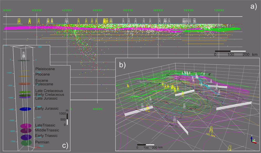
Figure 2. Geological data in GeoIT3D
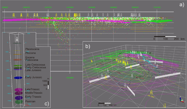
The pink lines are the isobaths of Adriatic Moho, the green lines are the isobaths of Tyrrhenian and European Moho, the yellow lines are the lithosphere isopachs, points of different colors represent hypocentres and magnitude of earthquakes (Figure 2a), white and yellow derrick are for deep wells of IEDM and DSDP/ODP respectively. The white lines indicate the position of the CROP seismic profiles (Figure 2b), light blue points indicate the position of the whole IEDM dataset (Figure 2b). a) North-south oriented view. b) Perspective view from SE. Five seismic images are visible. c) Visualization of chronostratigraphic data in Amanda 001bis well.
Table 2. Data stored in GeoIT3D
| 3D spatial data | cell size (m) | file format |
|---|---|---|
| DEM | 250 | ASCII |
| number | ||
| IEDM wells | 1.394 | ASCII |
| DSDP/ODP wells | 19 | ASCII |
| [number] (km) | ||
| CROP Project - interpreted sections | [4] (776) | bmp/dxf |
| number | ||
| CSI – earthquake hypocentres | 39.020 | ASCII |
| max depth/equidistance value | ||
| Base of Pliocene isobaths map | 9 km/500 m | dxf |
| Moho isobath maps | 56 km/2 km | dxf |
| Lithosphere thickness map | 130 km/20 km | dxf |
| cell size (degree) | ||
| Lithosphere-astenosphere system | 1°x1° | ASCII |
| number | ||
| Database of Individual Seismogenic Sources | 217 | ASCII |
| other spatial data | [number] (km) | file format |
| CROP Project - seismic lines on-shore | [17] (1,254) | bmp |
| CROP Project - seismic line off-shore | [46] (8,740) | bmp |
| number of measurement points | ||
| Heat flow | 2.700 | dxf |
| Gravity anomalies | 277,863 on-shore | dxf |
| 80,288 off-shore |
Two main data types are distinguished (Table 2):
1. 3D spatial data characterized by x, y, z or multiple z-value (spatial coordinates) and attributes (e.g. age, magnitude, lithostratigraphic unit, Vs, Vp, Density);
2. other spatial data characterized by x, y (spatial coordinates) and attributes as, for example, Two Way Times (sec), gravity anomalies (mGal), and heat flow (mW/m2). Although these data cannot be directly displayed in depth their informative content can be deployed by visualizing them as attribute on other geologic features (e.g., gravity anomalies map draped on the DEM).
The spatial data include also published maps elaborated by various authors (e.g., Moho and base lithosphere maps). As a matter of fact, these maps are characterized by complex interpolation of large quantities of data, but they supply either few or none information on the used interpolation method, and rarely provide data quality description. However these maps supply essential constraints for 3D modeling at depth.
Each modeled dataset are briefly describe here below, from the topographic surface to the deep lithosphere-astenosphere system.
3D spatial data
DEM
A digital elevation model (DEM) is used as reference for all the datasets collected in the 3D environment. The DEM (Italian Military Geographic Institute), deriving from a grid with a cell size of 250 meters, is a surface representing the hypsometry and the bathymetry for the Italian peninsula and surrounding offshore areas.
Deep wells for hydrocarbon and geothermal exploration
The Italian Economic Development Ministry (IEDM) collects and maintains all the information obtained from deep wells for oil, gas and geothermal exploration. Data related to wells no longer considered proprietary have been acquired by the SGI (Table 2), informatized and included in its databases.
Within GeoIT3D, in order to easily allow the comparison of data at national scale, only the chronostratigraphic information, corresponding to epoch boundary, are presented in each well using circles of different colors (Figure 2c). However, the original dataset contains more information including description of drilling cuttings, age of lithostratigraphic units, lithology description, attitude, mineralization, depositional environment, porosity, biostratigraphy, and gas percentage, and geophysical logs as, for example, electric potential (mV), resistivity (Ohm m2/m), sonic log (μsec/ft).
Unfortunately, the attitude data (azimuth and dip), which are an excellent constraint in 3D modeling, are only rarely available.
Digital deep well data are organized in ASCII files and include the following fields: x, y, z, azimuth, dip, and epoch. The mean depth is about 2,250 m, with maximum depth of 7,810 m.
Deep Sea Drilling Project/Ocean Drilling Project wells
Data from 19 wells located in the Mediterranean Sea and completed as part of the Deep Sea Drilling Project/Ocean Drilling Project (DSDP/ODP) have been acquired (Figure 2a/2b). Generally the whole dataset for each well contains the following data types: age profile, carbonate content, core depth recovery, density/porosity, grain size, gamma ray attenuation, nannofossils, ostracodes, site summary information, smearslide description, x-ray mineralogy (bulk, clay fraction, silt fraction).
For the purpose of GeoIT3D only the tables related to site summary information, age profile and core depth recovery have been extracted from the complete dataset for each hole (Kastens et al., 1990).
The data are organized in ASCII files with the following fields: x, y, z, azimuth, dip, epoch.
Base of Pliocene isobaths map
The isobaths map 1:500,000 scale representing the base of Pliocene deposits has been digitized from the Structural Model of Italy (CNR, 1992) and imported as a .dxf file.
The map has a 500 meter contour interval and represents the geometry of the base of Pliocene deposits in Padane-Adriatic foredeep.
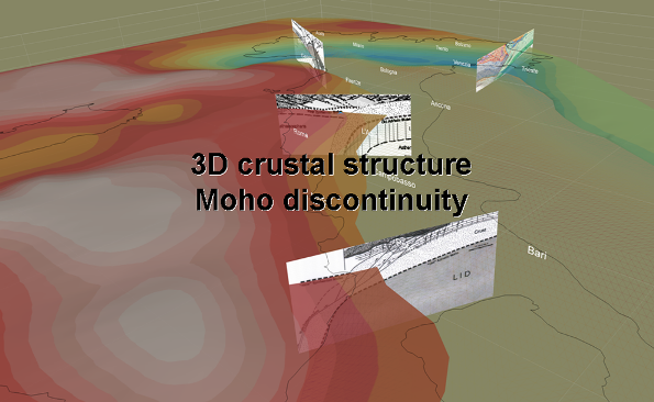
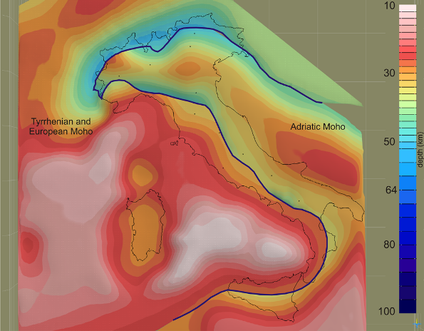
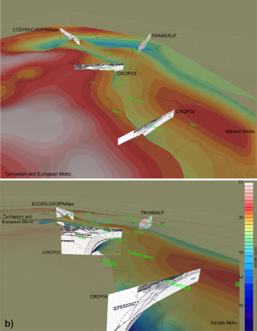
Figure 3. Moho discontinuity

Surfaces representing the Moho discontinuity resulting from the integration of Moho isobath maps and geological cross-sections based on CROP seismic profiles. b) in the foreground the underthrusting of the Adriatic Moho beneath the Tyrrhenian Moho (wireframe surface), in the background the Adriatic Moho overrode the European Moho (wireframe surface).
Moho isobath maps
Several interpretations of Moho-discontinuity isobaths have been proposed for the Italian area or for parts of it (Cassinis, 1983; Wigger, 1984; Nicolich, 1989; Nicolich & Dal Piaz, 1992; Nicolich, 2001). Updated interpretations for the Italian Alps (Kissling, 1993, Scarascia & Cassinis, 1997; Waldhauser et al., 1998) and for the Ligurian, Tyrrhenian and Ionian Seas and adjacent onshore areas (Scarascia et al., 1994) have been proposed.
One of the most recent reconstructions has been developed within the framework of the EUCOR-URGENT project (Dèzes & Ziegler, 2001) (see http://comp1.geol.unibas.ch and references therein). This map, with minor modifications derived from the interpreted CROP crustal reflection profiles, has been digitized and integrated into the GeoIT3D (Figure 2b).
CROP Project - interpreted sections
Four on-shore geological transects based on the interpretation and depth conversion of CROP seismic reflection profiles have been used to improve definition of the Moho surface.
Several interpretations of these CROP profiles have been proposed by various authors; in this project we have adopted the following interpretation: ECORS-CROP WAlps (Roure et al., 1996), TRANSALP (Castellarin et al., 2006), CROP03 (Carminati et al., 2004), and CROP04 (Scrocca et al., 2005).
The Moho position shown on these profile interpretations has been used as depth control on the modeled Moho surfaces (Figure 3 and Video “3D crustal structure”).
The data format is .bmp for the scanned images and .dxf for the digitized profiles.
Lithosphere Thickness map
The overall characteristics of the lithosphere-asthenosphere system, and their lateral variations, in Italy and surrounding regions were reconstructed during the 1980s (Calcagnile & Panza, 1980; Panza et al., 1980; Panza, 1984; Suhadolc et al., 1990).
The map of the lithospheric thickness, based on an analysis of surface wave dispersion, created by Panza et al. (1992) has been included in the database (Figure 2b).
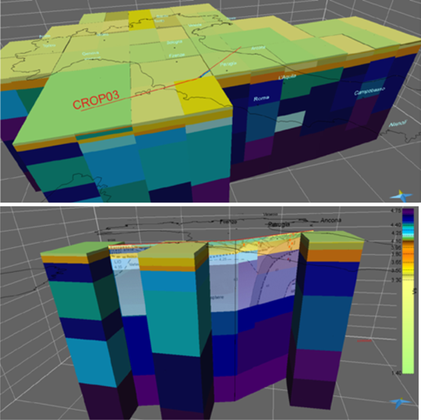
Figure 4. Lithosphere-astenosphere system

Volumes for the lithosphere-astenosphere system (cell 1°x1°) and geological cross-section along CROP03 (Carminati et al., 2004). The colour palette on the right is for Vs values.
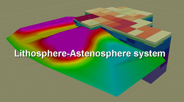
Afterward, in the frame of DPC-INGV Seismological Project S1, data obtained from surface wave tomography and non-linear inversion of dispersion curves, for 1° x 1° cells, in the whole Italic region (Brandmayr et al., this volume) are collected.
Starting from these data volumes characterized by the thickness (h), Vs, Vp and Density values assigned to the corresponding layer in the original dataset and describing the main characteristics of lithosphere-asthenosphere system are built (Figure 4 and Video “Lithosphere-Astenosphere System”).
Catalogue of Italian Seismicity
The Catalogue of Italian Seismicity (CSI1.1), for the period 1981 to 2002, contains 91,797 localized earthquakes of 136,850 recorded earthquakes and 39,020 magnitude estimates greater than 1.5 (Castello et al., 2006).
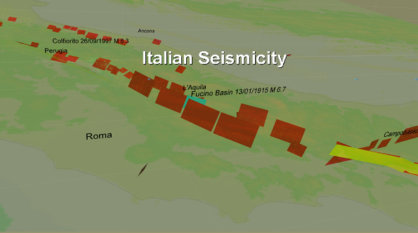
For the visualization in GeoIT3D (figure 2a, figure 5), only earthquakes with hypocentre deeper than 1 km and with a magnitude greater than or equal to 1.5 are shown (Video “Italian seismicity”).
The data are organized in ASCII file characterized by the following fields: x, y, z, magnitude.
Database of Individual Seismogenic Sources
The Database of Individual Seismogenic Sources - DISS (version 3.1), realized by INGV (Basili et al., 2008; DISS Working Group, 2009), has been modeled in three-dimension. The dataset contains 98 composite seismogenic sources (CS) and 119 individual seismogenic sources (IS) for the Italian region and surroundings areas (Video “Italian seismicity”).
Spatial attributes from DISS have been acquired to perform the 3D modeling of each seismogenic source (Figure 5). They consist of: coordinate pairs, depths of top edge and bottom edge, Rake (ranging from Min to Max for composite sources).
Figure 5. Italian seismicity
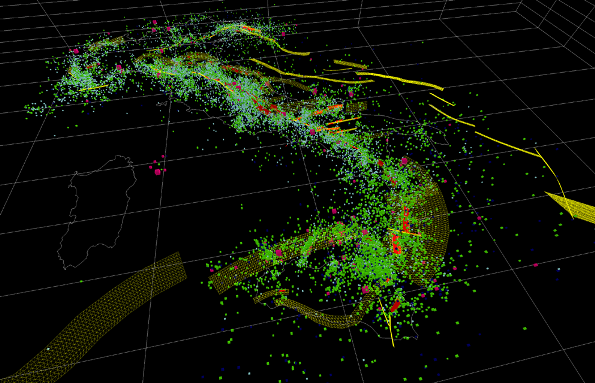
Distribution of the Italian seismicity and 3D modeling of seismogenic sources from DISS (CS – yellow; IS – red). The pink points represent earthquake with Magnitude > 4.
Other spatial data
CROP Project - seismic lines
Between 1986 and 1999, 9,800 km of seismic reflection profiles were recorded in Italy as part of the CROP Project. 17 on-shore (1,254 km) and 46 off-shore (8,740 km) seismic lines form the available dataset. Ranging from 10 to 25 sec (processed trace length), they were located to cross the most important structures of Italian land and sea and to provide definition of deep geological features (Scrocca et al., 2003).
The images (.bmp) of all seismic lines have been georeferenced and imported into GeoIT3D (Figure 2b, Figure 6).
Gravity anomalies
The Gravity map of Italy combines a very large number of gravity measurements: 277,863 on-shore and 80,288 off-shore stations. These gravity measurements were interpolated onto a square grid with a cell size of 1 km. The map shows gravity contours with a 10 mGal interval (Bouguer anomalies – on-shore stations; free air anomalies – off-shore stations) obtained following application of a square bidimensional gaussian filter operator to reduce local noise (APAT, 2005) and slightly smoothed (Video “3D crustal structure”).
Heat flow
The imported heat flow map was developed by processing 3,200 heat flow measurements collected from boreholes, tunnels, geothermal wells and hydrocarbon exploration wells, and in the upper 10 meters of the sea floor and lake sediments, scattered all over Italy and surroundings offshore areas (Della Vedova et al., 2001).
The digitized map has a contour interval of 20 mW/m2.
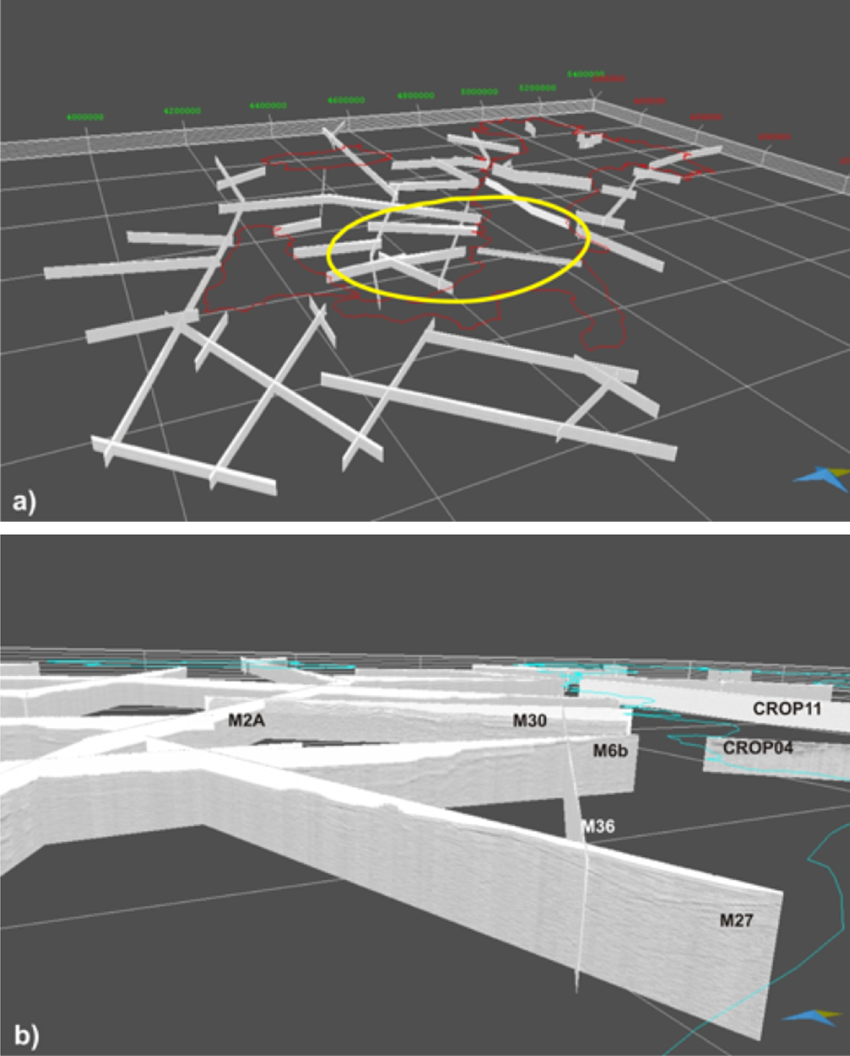
Figure 6. Seismic reflection profiles

a) Location of the CROP Project seismic profiles; b) a zoom of the lines into the yellow circle is shown (the vertical scale is time).
Three-dimensional modeling
Software
The software used to manage data and to construct 3D geological models is Move™ by Midland Valley Exploration Ltd.. This software package allows the integration of a wide range of datasets including outcrop data (stratigraphic boundaries, structural elements, attitudes), well and seismic data, and images.
Every object loaded in Move™ is composed of points and the geometric modeling is based on surfaces of a triangular network connecting and honouring all the selected data points. Different algorithms, useful for different type of datasets (dense, sparse or mix data), can be used to construct surfaces.
Move™ allows to honour the multi-scale approach proposed in this work combining, in a single 3D environment, different types of spatially referenced data from regional (e.g. Moho isobath maps) to larger scale (e.g. outcrop data or borehole stratigraphies), enabling the user to integrate data across a wide range of scales within a single comprehensive model.
The tools provided by the Move™ suite allow to perform specific operation such as: mapping the dilatation of an object due to deformation (strain analysis), measuring the curvature on a surface (curvature analysis), measuring the average cylindrical vector of a folded surface (cylindrical analysis), etc..
Additional analysis for structural restoration and forward modelling can be applied with the specific tools available in Move™.
Moreover specific operations are enabled in the 3D environment to create and analyse volumes.
Regional 3D modeling
Move™ has been used to integrate the full suite of available national-wide data and to generate geological surfaces and volumes that provide an overview of the deep structure in the Italian region. Some of the datasets (deep wells, CSI) enable the user to check the shape and the spatial relationships between the main modeled features and to verify their consistency with geophysical data (gravity anomalies, heat flow).
The constructed 3D surfaces are the base of Pliocene deposits for the Padane-Adriatic foredeep, the Moho discontinuity (Figure 7), and the base of the lithosphere.
These surfaces have been generated using the model building tool (Tessellation algorithm) of 3DMove, which faithfully honours all of the data points from the selected dataset; furthermore each surface has been resampled, using a grid interval with order of magnitude comparable with its maximum depth, to obtain an homogeneous distribution of quoted points, more useful for future analyses.
The results are encouraging, although data density decreases with increasing depth, and surface definition in deeper maps is less precise than in shallower ones.
Figure 7. Base of Pliocene deposits and Moho surfaces (perspective view from SW)
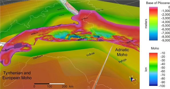
The highly irregular surface, from pink to blue, is the base of Pliocene deposits; the yellow to green surfaces are the Adriatic Moho and Tyrrhenian-European Moho (translucent). Images of interpreted seismic profiles are partially visible. The base of lithosphere is not visible here.
The surface representing the base of Pliocene deposits in the Padane-Adriatic foredeep has been obtained from the isobaths map of the Structural Model of Italy (CNR, 1992). The shape and the geometry of this feature have been verified using the constraints from stratigraphies of deep wells.
A grid interval of 1,000 meters has been applied to the modeled surface (Figure 8), where steep morphologies locate the main structural elements.
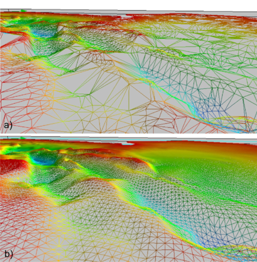
Figure 8. Modeling of the base of Pliocene deposits

a) original base of Pliocene deposits surface derived from isobaths; b) resample of the original surface; the steep morphologies, corresponding to the main structural elements, are preserved.
3D reconstruction of the Moho discontinuity are based on isobath data and include some interpreted and depth converted CROP seismic reflection profiles.
The basic framework of the Moho discontinuity is clearly displayed in GeoIT3D (Figure 9 and Video “3D crustal structure”) and supports the following observations.
a. Several different Moho discontinuities may be distinguished: 1) a new forming Neogene-Quaternary Moho with low velocities in the Tyrrhenian basin and Western Apennines (Tyrrhenian Moho), 2) an old Paleozoic-Mesozoic Moho in the Padano-Adriatic-Iblean foreland areas (Adriatic Moho), and 3) another Paleozoic-Mesozoic old Moho in the Alpine belt and Sardinia (European Moho).
b. The Italian crust is generally continental, except in the Tyrrhenian abyssal plain, where a 10 km thick Late Miocene - Pliocene oceanic crust is present, and in the Ionian Sea, where a Mesozoic oceanic crust is buried underneath a thick pile of sediments (Catalano et al., 2001).
c. Stable areas (Sardinia, Adriatic sea and Apulia) have Moho depths of about 30 km, while the crust is thicker underneath the Alpine belt (45-55 km) and thinner in western Tuscany and Latium (20-25 km).
d. The Adriatic Moho overrode the European Moho in the Alps, while underthrusting of the Adriatic Moho beneath the Tyrrhenian Moho occurred along the Apennines.
Similarly, the main features of the lithosphere-asthenosphere system can be easily recognised. The lithospheric thickness in foreland areas varies from 70 km in the Northern Adriatic Sea to about 110 km in the Apulian domain to the southeast. In the Tyrrhenian Sea, the lithosphere thins to 20-30 km, while to the north, its thickness increases approaching 130 km in the Western Alps. The distinction between the new lithosphere in the Tyrrhenian back-arc basin and the old, subducting Apulo-Adriatic lithosphere has not been represented in this reconstruction.
Data can be extracted from the 3D model in a variety of forms including cross-sections, contour maps, grids, etc.. As an example a section cutting across the northern Apennine, from Ferrara to Livorno (Figure 10), has been produced which displays all the different data types collected and modeled in GeoIT3D, supporting the validation of data interpretation.
Figure 10. Geological cross-section

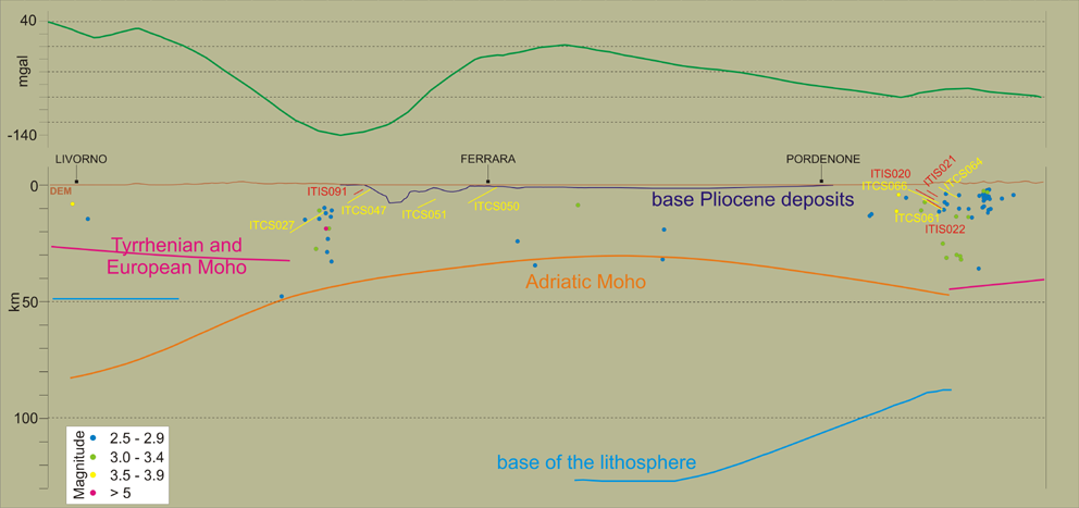
Geological cross-section from the Tyrrhenian Sea (Livorno) to the Western Alps (Pordenone) deriving from the datasets stored in the 3D environment. The green curve represents the gravity anomalies along the section.