Methodology
Surface wave dispersion data and tomography
The surface wave dispersion data are used in the present study to investigate the VS structure in the Italic region. The following methods are applied in the sequence: (a) frequency-time analysis, FTAN (Levshin et al., 1989, and references therein), to measure group-velocity dispersion curves of the fundamental mode of Rayleigh waves; (b) two-dimensional tomography (Yanovskaya, 2001, and references therein) to map the distribution of group and phase velocities of Rayleigh waves, plotted on a grid 1°×1° to compile the cellular dispersion curves; (c) non-linear inversion (Panza, 1981, and references therein) of the assembled cellular dispersion curves to calculate the set of accepted models for each cell; (d) smoothing optimization algorithms (Boyadzhiev et al., 2008) to choose the representative model for each cell and thus to define, for the Italic region, the three-dimensional VS model and its uncertainties.
The FTAN is an interactive group velocity-period filtering method that uses multiple narrow-band Gaussian filters and maps the waveform record in a two-dimensional domain: time (group velocity) -frequency (periods). The measurement of group velocity of Rayleigh and/or Love waves is performed on the envelope of the surface-wave train and can be robustly measured across a broad period band, from fractions of seconds to hundreds of seconds (e.g. Chimera et al., 2003; Guidarelli and Panza, 2006). Seismic records from national and international seismic networks are analyzed by FTAN to study the velocity structure in the broad Mediterranean region. The information about the hypocenters of the events (location, depth, and origin time) is collected from NEIC (2003) or ISC (2007). The length of most of the epicenter-to-station paths considered does not exceed 3000 km in order to have, as much as possible, reliable measurements of group velocity at short and intermediate periods. After group-velocity measurements, all the curves are linearly interpolated and sampled at the set of predefined periods. In addition group-velocity measurements available in the literature have been considered. The penetration depth of our dataset is increased (Knopoff and Panza, 1977; Panza, 1981) considering published phase-velocity measurements for Rayleigh waves that span over the period range from about 15 s – 20 s to about 150 s.
The two-dimensional tomography based on the Backus–Gilbert method is used to determine the local values of the group and/or phase velocities for a set of periods, mapping the horizontal (at a specific period) and vertical (at a specific grid knot) variations in the Earth's structure. From these tomographic maps, local values of group and phase velocities are calculated on a predetermined grid of 1°×1°, for a properly chosen set of periods, in the ranges from 5 s to 80 s for group velocities and from 15 s to 150 s for phase velocities. The choice of the set of periods is based on the vertical resolving power of the available data, as determined by the partial derivatives of dispersion values (group and phase velocities) with respect to the structural parameters (Panza, 1981). The lateral resolution of the tomographic maps is defined as the average size, L, of the equivalent smoothing area and its elongation (Yanovskaya, 1997) and hence it is not necessary to perform check board or similar tests.
The local dispersion curves are assembled at each grid knot from the tomographic maps. The average size L and its stretching is used as a criterion for the assemblage of the local dispersion curves. At each period, the group and/or phase velocity value is included in the dispersion curve if L is less than some limits: for group velocity Lmax is 300 km at the period of 5 s and increases to 600 km at 80 s; for phase velocity Lmax is 500 km at the period of 15 s and reaches a value of 800 km at 80 s; the stretching of the averaging area of all considered values is less than 1.6. Hence the local dispersion curves have a different period range and take into account only the dispersion values sufficiently well resolved.
Each cellular dispersion curve is calculated as the average of the local curves at the four corners of the cell. The single point error for each value at a given period is estimated as the average of the measurement error at this period and the standard deviation of the dispersion values at the four corners. If, at a given period, the cell is crossed by few wave paths, and, according to the Lmax criterion, the dispersion value at a corner of the cell is not available, the value of the single point error is doubled. The value of group velocity at 80 s is calculated as an average between our tomography results and the global data from the study of Ritzwoller and Levshin (1998). The single error at this period for group velocity is estimated as the r.m.s. of the errors of our data and those of the global data set. The r.m.s. for the set of dispersion curves (group or phase velocity) are routinely estimated as 60-70% of the average single point error of the specific cellular curve (Panza, 1981; Panza et al., 2007a). The assembled cellular dispersion curves span over a varying period range according to the available reliable data.
The non-linear inversion
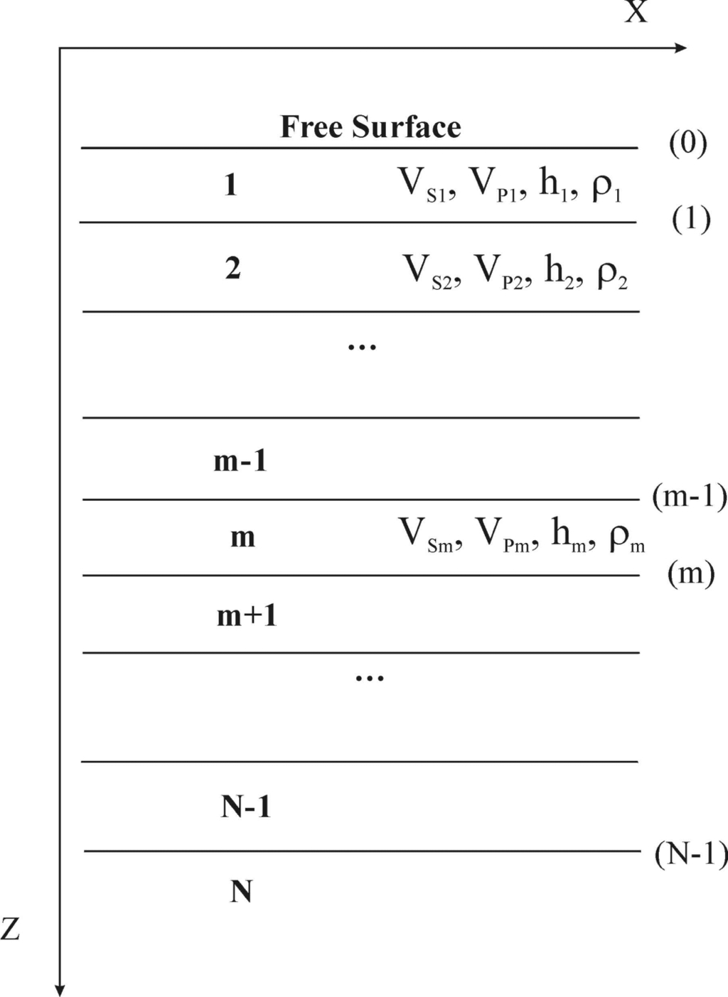
The non-linear “hedgehog” inversion method is applied to obtain the VS models for cells sized 1°×1° in the Italic region using the compiled cellular dispersion curves. To solve the inverse problem, the structural model of each cell has to be replaced by a finite number of numerical parameters, and, in the elastic approximation, it is divided into a stack of homogeneous isotropic layers (Fig. 1).
Figure 1. Earth’s model adopted for the inversion scheme.

The modeling of the Earth’s structure in hedgehog inversion by laterally-homogeneous isotropic plane layers. The physical properties VS, VP, thickness (h), density(ρ) of each layer can be independent (i.e. the variable parameters that can be well resolved by the data), dependent (i.e. in some fixed relation with inverted parameters) or fixed (i.e. during the inversion the parameter is held constant accordingly to independent geophysical evidence). Upper crust layers (i.e. layers 1, 2, …) are fixed according to independent data. Parameterized layers (i.e. layers m-1,..., m+1) are inverted, while the deep structure (i.e. layers N-1, N, …) are fixed according to global models.
The method is a trial-and-error optimized Monte Carlo search and the layer parameters (thickness, VP, VS, and density ρ can vary or be constant during the inversion procedure. For each dispersion curve, digitized at N points, the parameter’s steps δPj (where j is the number of parameters, equal to 10 in our case) are defined following Knopoff and Panza (1977) and Panza (1981) and they are minima subject to the condition:
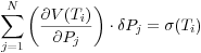 |
(1) |
where V(Ti) is the group or phase velocity at period Ti and σ(Ti) is the relevant standard deviation. The uncertainties of the accepted model are defined as ± half of the relevant parameter’s step.
The group and phase velocities of the Rayleigh waves (fundamental mode) are computed for each tested structural model. The model is accepted if the difference between the computed and measured values at each period are less than the single point error at the relevant period and if the r.m.s. values for the whole group and phase velocity curves are less than the given limits.
The structure is parameterized taking into account the resolving power of the data and a priori geophysical information. The resolving power of dispersion measurements is only indirectly connected with the lateral variations of the structural models and identical dispersion properties do not necessarily correspond to equal structures (see Appendix A). A priori independent information about the crustal parameters of each defined cell can be introduced in the inversion procedure to improve the resolving power of the tomographic data (Panza and Pontevivo, 2004; Pontevivo and Panza, 2006). A similar conclusion is reached by Peter et al. (2008): in the absence of an accurate crustal model, the retrieved upper mantle structure is dubious down to about 200 km of depth.
According to the values of the partial derivatives of the group and phase velocities for Rayleigh waves with respect to structural parameters (Urban et al., 1993), the assembled cellular dispersion data, in the period ranges from 5 s to 150 s for group velocity and from 15 s to 150 s for phase velocity, allows us to obtain reliable velocity structure in the depth range from 3 km – 13 km to about 350 km. In each cell, the Earth's structure is modeled by 19 layers down to the depth of about 600 km: the uppermost five layers have properties fixed a priori, using independent literature information specific for each cell; the following five layers have variable VS, VP, thicknesses and if necessary - density; in the eleventh layer VP, VS, and density are fixed while the thickness varies in such a way that the whole stack of eleven layers has a total thickness, H, equal to 350 km; below 350 km of depth there are eight layers, of Poissonian material, with constant properties common to all cells. The structure below 350 km is taken from the average model for the whole Mediterranean, EurID database, of Du et al. (1998). The EurID database is based upon existing geological and geophysical literature, it incorporates topographic and bathymetric features and it has been proven to be quite consistent with several broad-band waveforms. The use of global models, e.g. ak135 (Kennett et al., 1995), for the structure below 350 km does not introduce any significant difference in the calculated dispersion curves (Raykova and Panza, 2010), thus does not affect our inversion results. In each cell, the thickness of the fixed uppermost crustal structure depends on the lower limit of the period range of the cellular dispersion curves, and varies from about 3 km to 13 km. When the cell is located in a sea region, the thickness of the water layer is defined as a weighted average of the bathymetry and topography (on-line data from NGDC, 2003) inside the area of the cell. The thickness of the sediments is defined in a similar way from the map of Gennesseaux et al. (1998) or from the data given by Laske and Masters (1997). The structural data available from seismic, geophysical and geological studies in the region are used to fix the properties of the remaining upper crustal layers. The same information is considered in the parameterization of the five layers used to model the depth range from 3 km – 13 km to 350 km. Eleven parameters (Pj, j=1,10 and P0) are used to define these five layers: five for the shear-wave velocity in each layer, five for the thickness of each layer, and P0 for the VP/VS ratio. The independent available geophysical information is used to define the following parameters ranges: (1) Moho depth; (2) VS in the crust (VS ≤ 4.0 km/s); (3) VS in the mantle layers (4.0 km/s ≤ VS ≤ 4.8 km/s); (4) the total thickness of the parameterized structure cannot be greater than 350 km (the maximum depth of relevant penetration of our data). Nevertheless, the VS ranges for crust and mantle represent globally valid rules that may not be satisfied in some specific complex cases. In the Alps, the maximum VS in the crust is set to 4.10 km/s according to reported velocities for some crustal minerals (Anderson, 2007) and in the upper mantle beneath Tyrrhenian Sea, where a high percentage of melting is present (Panza et al., 2007a), low mantle velocities (VS ≤ 4.0 km/s) are allowed.
Optimization algorithms
The non-linear inversion is multi-valued and a set of models is obtained as the solution for each cell. In order to summarize and define the geological meaning of the results, it is necessary to identify a representative model, with its uncertainties, for each cell. An optimized smoothing method, which follows the Occam’s razor principle, is used to define the representative model for each cell with a formalized criterion. This method avoids, as much as possible, the introduction of artificial discontinuities in VS models at the borders between neighboring cells and keeps the 3D structure as homogeneous as possible by minimizing the lateral velocity gradient. In this way, the dependence of the final model from the predefined grid is minimized. The method represents the models as velocity vectors with equal size (250 layers) for all sets of cellular solutions. The distance (divergence) d between two models (velocity vectors) w and v is defined as the standard Euclidean norm between two vectors:
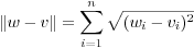 |
(2) |
where wi and vi are the S-wave velocities in the ith layer and n is the number of layers in the models.
To take into account the contribution of the ith layer thickness, each velocity value has been weighted with the ratio given by the correspondent layer thickness, h, over the total thickness of the structure, i.e. in the ith layer the weighted velocity (vWi) is:
 |
(3) |
Three quite different criteria for optimization have been developed that lead to the minimization of the lateral velocity gradient for the whole domain, or, in other words, to the smoothing of the shape of the global solution in all the study area Ω as much as possible.
The definitions of the criteria are as follows. (I) Local Smoothness Optimization (LSO): the optimized local solution of the inverse problem is the one that is searched for, cell by cell, considering only the neighbors of the selected cell and fixing the solution as the one which minimizes the norm between such neighbors. (II) Global Flatness Optimization (GFO): the optimized global solution of the inverse problem with respect to the flatness criterion is the one with minimum global norm in-between the set of global combinations G(Ω). (III) Global Smoothness Optimization (GSO): the optimized global solution of the inverse problem with respect to the smoothness criterion is the one with minimum norm in-between all the members of the subset Γ(Ω).
The LSO follows the principle of minimal divergence in the models. The search starts from the cell where the average dispersion of the cellular models is minimal, i.e. the accepted solutions in this cell are the densest in the parameter space and therefore the potential systematic bias introduced by the choice is minimized. The LSO fixes, as the representative solution of the processed cell δi,j, the cellular model that minimizes the norm between the neighbour cells δi±1,j±1 (i.e. cells with one side in common). Once a solution is chosen in the running cell, it is fixed and the search continues by applying the procedure to one of the neighbouring cells, not yet processed, and with the smallest average dispersion of the cellular models. The LSO follows the direction of “maximum stability” in the progressive choice of the representative solution of the cells until the whole investigation domain is explored.
The GSO is based on the idea of close neighbours (local smoothness) extended, in a way, to the whole study domain. The method consists of two general steps. The first step extracts a suitable subset Γ(Ω) from G(Ω), namely the global combination u belongs to Γ(Ω) if and only if:
 |
(4) |
where ũ ∊ δi±1,j±1. In other words Γ(Ω) contains all global combinations with close neighbouring components. Then we select, as the best solution in G(Ω) with respect to the smoothness criteria, the member of Γ(Ω) with least global norm, i.e. we apply the flatness criterion to Γ(Ω) and not to the entire G(Ω).
The GFO is based on the concept of maximum flatness among the whole domain Ω. It records, by iterative steps for every row starting from the right border of the domain Ω, each combination of solutions in the processing row which has minimal norm with the combinations in the previous processed row. Then, in the last step, GFO selects the combinations which have the minimal global norm, with respect to flatness criterion, among the global set G(Ω).
Due to the different way of action and computing time necessary to perform GFO and GSO, we applied the three smoothing algorithms hierarchically in the region of Alps (Boyadzhiev et al., 2008). We perform LSO and GSO, which are the fastest methods acting on the smoothing criterion basis, on the whole area of the Alps. The application of these two methods preserves some local features which may be flattened by GFO, according to its acting criterion. Then, in order to reduce the dependence from the starting cell that affects LSO, the common solution to LSO and GSO are selected and fixed during the performed GFO. This sequential execution of the smoothing algorithms reduces the computing time and concentrates the effort on that portion of Ω in which the solutions chosen by LSO and GSO differ.
Since the non-linear inversion and its smoothing optimization guarantee only the mathematical validity of the solution of the inverse problem, the optimization procedure can be repeated whenever necessary, including additional geophysical constrains, such as Moho depth, seismic energy distribution versus depth, presented magmatism, heat flow, etc., until the appraisal of the selected models against well-known and constrained structural features gives a result comparable with the model’s uncertainties (see section “Discussion”).
The resulting three-dimensional VS structure of the study region is juxtaposed against the selected representative one-dimensional cellular models. The steps used in the parameterization of the non-linear inversion obey condition (1), therefore they can be used to define the uncertainties of each cellular model (Panza et al., 2007a). The representative cellular solution gives, for each inverted layer, the preferred value of VS and thickness with uncertainties equal, as a rule, to ±1/2 of the relevant parameter (VS or thickness) step. The a priori information is taken into account when the uncertainties of the representative solution are specified. Therefore, the variability range of the inverted parameters can turn out to be smaller than the step used in the inversion and the exact value given by the representative solution does not necessarily fall in the middle of its uncertainty range.
Independent geophysical constraints
The resulting representative cellular models are appraised and constrained using independent studies concerning Moho depth (Dezes and Ziegler, 2001; Grad and Tiira, 2008; Tesauro et al., 2008), seismicity-depth distribution (ISC, 2007), VP tomographic data (Piromallo and Morelli, 2005) and other independent information as the heat flow (Hurting et al., 1991; Della Vedova et al., 2001) and gravimetric anomaly (ISPRA, ENI, OGS, 2009).
The data from Dezes and Ziegler (2001), Tesauro et al. (2008), and Grad and Tiira (2008) are used to define the range of Moho depth for each cell. The Moho depth, with its uncertainties, is compared for each cellular model with the depth range derived from the literature. Where the value indicated by our models is out of the range, additional constraints are used (see section “Discussion”).
The depth distribution of seismicity is used as an additional criterion for appraisement of the cellular models. The revised ISC (2007) catalogue for the period 1904–June 2005 is used and for each cell we compute several histograms, grouping hypocentres in depth intervals. The depth grouping considers the uncertainties of the hypocentre’s depth calculation: 4 km for the crustal seismicity and 10 km for the mantle seismicity. The computed histograms are the following: (a) distribution of the logarithm of earthquake’s number per depth intervals (logN-h): (b) distribution of the logarithm of total energy released by the earthquakes per depth intervals (logE-h); (c) distribution of the logarithm of product of energy released by the earthquakes per depth intervals (log∏E-h). Each of these three depth distributions is generated for two selections of the events: all events in the considered catalogue and all events with depth not fixed during hypocenter calculations in order to reduce the influence of “standard” depths, as 33 km, in the histogram construction. The logN-h distribution gives an estimation of the material fragility in the relevant depth interval: high earthquake’s frequency is related to more brittleness materials. Similar distributions are used in the studies of Meletti and Valensise (2004) and Ponomarev (2007) but this kind of earthquake frequency distribution does not evidence the presence of strong single events. The logE-h distribution valuates the strangeness of the material in the relevant depth interval: high energy release is relevant to high energy accumulation in strong materials. This kind of seismic energy distribution is used by Panza et al. (2007a) but some strong badly located events can bias the results. The log∏E-h distribution gives an integral characteristic of the seismicity in the relevant depth interval, since the product of energy is proportional to the number of earthquakes and relevant energy release. Let us consider two events in a depth interval, with energy release of E1 and E2 respectively, where E1=aE2. The log∏E for this interval is the following:
 |
(5) |
The seismicity distribution presented in this way is used by Panza and Raykova (2008) to define the Moho depth in the Italic region.
The logN-h distribution is calculated using all events from ISC catalogue (with and without depth estimated). For energy calculation (logE-h and log∏E-h) the relation of Richter (1958) logE = 1.5MS + 11.4 is used considering all events from ISC catalogue with indicated magnitude. The value of MS is either directly taken from the ISC catalogue or computed from currently available relationships between MS and other magnitudes (Peishan and Haitong, 1989; Gasperini, 2002; Panza and Raykova, 2008). Some examples for computed seismicity-depth distributions are shown and discussed in section “Discussion”.
The information about heat flow (Hurting et al., 1991; Della Vedova et al., 2001) is used to define the nature of some relatively shallow layers (down to about 80 km of depth). A high heat flow likely indicates the presence of magma reservoirs with low VS at shallow depths. A low heat flow usually requests cold mantle (relatively high VS) and thick crust.
Independent information about gravimetric anomaly (ISPRA, ENI, OGS, 2009) together with heat flow data is used in the interpretation of the lithosphere-asthenosphere structure along several sections (see section “Discussion”).
The VP tomographic data of Piromallo and Morelli (2003) are used to reduce the uncertainty range of our VS models in the construction of the cellular database.
Non-linear inversion of moment tensor: INPAR method
The determination of the moment tensor, i.e. of the source mechanism of a seismic event from its complete waveforms, is a non-linear problem. Nevertheless, its determination is of fundamental importance to determine the properties of seismic sources, and straightforward for the comprehension of the local stress field acting in a given tectonic region.
Several methods were developed, linear and non-linear, from body waves, surface waves or complete waveforms, from a regional or global event. Some of them are routinely applied and published in bulletins shortly after a seismic event. However, all these methods have different accuracies and resolving power.
We analyze, in detail, the non-linear method named INPAR (INdirect PARameterization), developed at the Department of Geosciences, University of Trieste (Sileny et al., 1992; Sileny, 1998).
The INPAR method for the inversion of moment tensor, that adopts a point-source approximation, is a sophisticated non-linear method using the dominating part of complete waveforms from events at regional distances (up to 2500 km), in this way maximizing the signal-to-noise ratio. It consists of two steps, the former linear, the latter non-linear.
The kth component of displacement at the surface determined by equivalent forces in the point-source approximation is the convolution product of moment tensor and Green’s function spatial derivatives (Aki and Richards, 1980):
 |
(6) |
The Green’s functions represent the response of the medium to singlet sources with Dirac-delta time dependence.
In the first step, Green’s functions are extracted from signals to calculate the time derivatives of the six independent components of the moment tensor (hereafter MTRF) (Panza, 1985; Florsch et al., 1991; Panza et al., 2000), in this case with a time dependence given by Heaviside (step) function. Computing the MTRFs from Green’s functions does not require an a priori source model. Since a bad location of the focus may strongly affect the results of the inversion, INPAR performs, whenever necessary, a re-location of the focus within a fixed volume around the available location. For intermediate coordinates within this volume the base functions, i.e. the medium response to a seismic source modeled by an elementary single source with the time dependence given by Heaviside function, are computed interpolating the base functions computed at the corners of the volume itself. From base functions, the synthetic seismograms are computed and are compared with observed ones: the L² norm of synthetic and observed seismograms is minimized to determine the new focus location.
In the next non-linear step, the MTRFs are factorized in a time constant moment tensor mij and a corresponding source time function f(t):
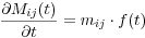 |
(7) |
assuming the same time dependence for all moment tensor components, i.e. a rupture mechanism constant in time.
The “predicted” values of the MTRFs, mij・f(t), are matched to the “observed” MTRFs (obtained as the output of the first step of the procedure). Thus, by introducing MTRFs in the first step, the problem of matching the seismograms is transformed to the problem of matching the MTRFs. This allows the reduction of the equations system for the searched source parameters, since the MTRFs are always six, while seismograms can be more than six. In order to reduce the errors coming from the poor knowledge of the structural inhomogeneities of the epicenter-station profile, which can cause scattering, only the correlated parts of the MTRFs are taken into account (Kravanja et al., 1999).
Additional constraints, such as the positivity of the source time function and, whenever available, consistency with polarities, are posed. After several iterations, the focal mechanism is obtained and reduced to the best double couple in case of tectonics events. In this way the volume components, which are often artefacts of the inversion process, are discarded (Kravanja et al., 2000).
INPAR is particularly suitable for determining the foci of shallow events, due to the possibility to use waveforms of relatively short period (down to 10 s). Theoretically, the seismic moment tensor cannot be univocally determined from surface waves signals whose wavelength significantly exceeds the source depth (Bukchin and Mostinskii, 2007), since two components of the moment tensor, Mzx and Mzy, excite a Green’s function vanishing at the free surface. Because of this, the CMT and RCMT methods, which respectively use body and surface waves at periods greater than 35 s, usually fix shallow events at depths of 10 km the former and 15 km the latter.
The correct determination of the hypocentral parameters of a tectonic event is of crucial importance for a reliable understanding of the geodynamic context in which the event occurred. The information coming from moment tensor inversion can be inserted in the tectonic picture obtained from tomography to better constrain it (see section “Discussion”).
Further development: cellular database
A cell-by-cell database has been compiled to compare the obtained results with some independent data (VP, attenuation and density) to enable an easier way to access the data. All collected information for each cell is stored in a table. An example of the database for cell 42.5N 13.5E (b3, L’Aquila) is given in Table 1.
The VP data are taken from Piromallo and Morelli (2003) where a P-wave tomography study of the whole Mediterranean region is provided on a grid of 50 km in both horizontal and vertical directions down to a depth of 1000 km. The VP data are given in a coordinate system which is rotated with respect to the geographical one. The prime meridian in the rotated system is 10° W, while the “rotated equator” is the great circle crossing the prime meridian at 45° N. To complete our database, the VP data are averaged to obtain a single set of VP values for each of our 1°×1° cells. The averaged data are interpolated linearly to obtain the value of VP at the centre of each layer of our cellular structures. The VP data are considered only for the mantle layers down to a depth of 350 km, as the considered P-wave tomography poorly resolves the upper crustal structure.
The calculated VP value for each layer in our cellular models permits to reduce the uncertainty ranges of VS in the mantle, as far as the VP/VS ratio in the mantle is kept as close as possible to 1.82 (Kennett et al., 1995).
The density data are taken from Farina (2006) where the gravity inversion method is applied to model the density along a set of sections in the Italic region and surroundings. About 30% of our cells are not modelled by Farina (2006). The densities in some of these cells are obtained by linear interpolation of the density in the neighbouring cells (e.g. cells C3, B6, A5). Where the interpolation was not possible, the density data are those used as fixed input in the non-linear inversion.
The database is completed with S-wave attenuation (QS) data given in the recent studies of Martinez et al. (2009, 2010) for the Mediterranean at latitude less than 45°N. Using averaging and linear interpolation, the value of QS is calculated for the centre of each layer in our cellular solutions. The QS data for the rest of the cells are taken from Craglietto et al. (1989). The values of P-wave attenuation (QP) has been derived using the relation QP= 2.2QS (Anderson, 2007). All VP and VS values are rounded to 0.05 km/s, according to the precision of our modelled data.
In some cases a VS inversion is modelled in the upper 20 km. Whether this is a real structural feature or an artefact of the inversion will be a matter to be settled performing the inversion using the receiver functions data to better constrain the upper fixed crust.
Table 1. Cellular database
| H | ρ | VP | VS | QP | QS | Z | Lon | Lat | ΔVS+ | ΔVS- | ΔH+ | ΔH- | VP/VS |
|---|---|---|---|---|---|---|---|---|---|---|---|---|---|
| 1.2 | 2.30 | 2.70 | 1.55 | 440 | 200 | 1.20 | 13.50 | 42.50 | 0.00 | 0.00 | 0.00 | 0.00 | 1.74 |
| 0.8 | 2.50 | 3.70 | 2.13 | 418 | 190 | 2.00 | 13.50 | 42.50 | 0.00 | 0.00 | 0.00 | 0.00 | 1.74 |
| 1.5 | 2.60 | 5.35 | 3.10 | 418 | 190 | 3.50 | 13.50 | 42.50 | 0.00 | 0.00 | 0.00 | 0.00 | 1.73 |
| 12.0 | 2.75 | 5.70 | 3.30 | 330 | 150 | 15.50 | 13.50 | 42.50 | 0.05 | 0.05 | 1.50 | 1.50 | 1.73 |
| 20.0 | 2.80 | 6.40 | 3.70 | 198 | 90 | 35.50 | 13.50 | 42.50 | 0.15 | 0.10 | 5.00 | 5.00 | 1.73 |
| 60.0 | 3.30 | 7.90 | 4.40 | 176 | 80 | 95.50 | 13.50 | 42.50 | 0.15 | 0.00 | 0.00 | 15.00 | 1.80 |
| 60.0 | 3.30 | 8.00 | 4.35 | 176 | 80 | 155.50 | 13.50 | 42.50 | 0.00 | 0.15 | 25.00 | 0.00 | 1.84 |
| 110.0 | 3.30 | 8.70 | 4.60 | 220 | 100 | 265.50 | 13.50 | 42.50 | 0.00 | 0.20 | 0.00 | 25.00 | 1.89 |
| 84.5 | 3.60 | 8.95 | 4.75 | 330 | 150 | 350.00 | 13.50 | 42.50 | 0.00 | 0.00 | 0.00 | 0.00 | 1.88 |