The Upper mantle
The topography of Asia is dominated by the results of Indo-Eurasian continental collision still continuing apace at ~5 cm/yr (Paul et al. 2001). Large scale tectonics on earth is constrained by the behavior of the outer brittle lithospheric caps or plates in response to the heat transfer from the interior. A consideration of the thermo-mechanical properties of the entire cratonal lithospheres inclusive of their crusts is, therefore central to understanding the structure and evolution of the Indian shield. Studies of mantle nodules geochemistry, especially of the diamondiferous, have shown that several cratons have lithospheric roots as deep as 250km. Rayleigh wave dispersion curves which are sensitive to the shear wave structure in the vertical plane containing the source-receiver path, allow one to determine average Rayleigh wave phase and group velocities in this plane at various periods, each with their characteristic peak depth sensitivities at approximately a third of the wavelength. With a sufficient number of such intersecting source receiver paths available, these observations allow one to perform a tomography of the region under study in 3 dimensions, and inversions thereof in terms of the shear wave speed structure of the mantle lithosphere to shed light on its temperature regimes.
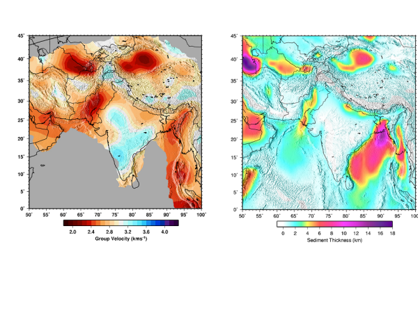
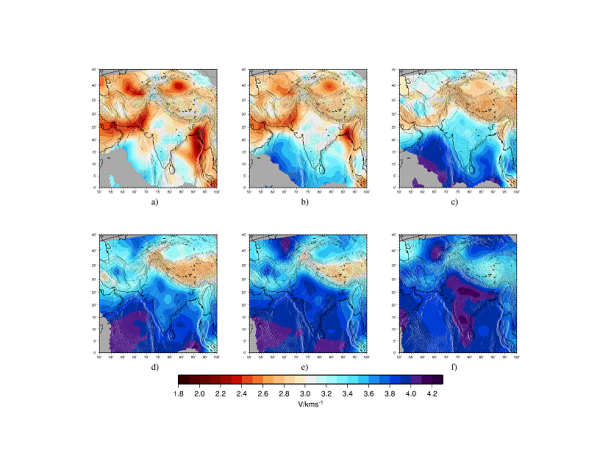
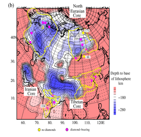
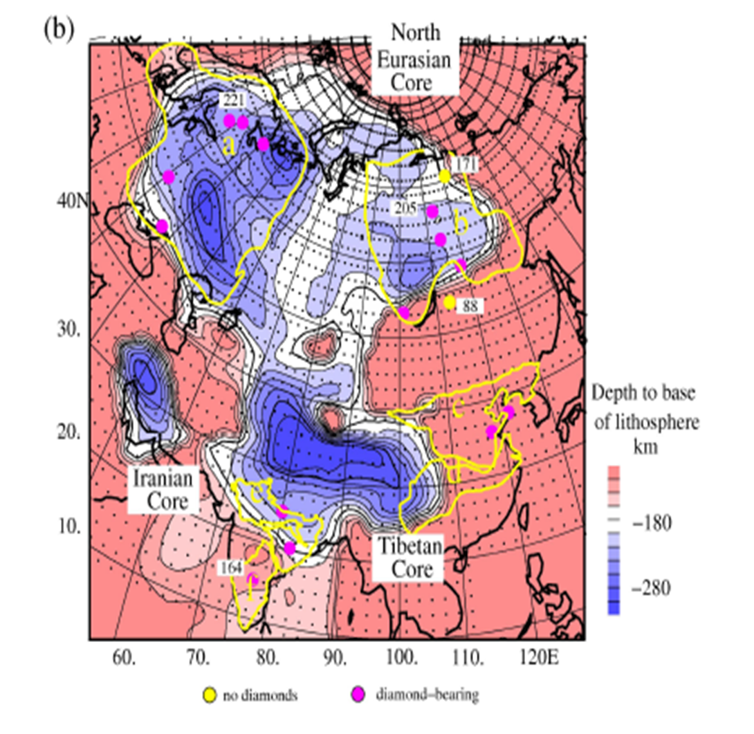
Results of a recent such analysis (Charlotte Acton, 2009) based on 4054 source-receiver paths covering most of India and Tibet, are shown as group velocity maps in Figure 6 for the 10 sec period and in Figure 7 for a few longer periods (15,20,30,40,50,70 seconds) constrained to a lateral resolution of 3-5º. The 10 seconds map (depth sensitivity of ~12km) clearly highlight the low velocity areas occupied by prominent sedimentary basins: the Tarim basin in Tibet, the Katwaaz basin in Pakistan, as well as the Himalayan foredeep and the Bengal basin, virtually reproducing Laske’s (1997) sediment thickness map shown on the right. It also maps the 5 cratonic exposures as contiguous higher velocity areas little distinguished from the intervening mobile belts. Whilst Tibet remains hot down to 70km, the strong signatures of the sedimentary basins progressively disappear at around mid-crustal depths (~20 sec. period) even as the cratons begin to acquire sharper outlines coalescing their roots at ~100km (70 sec period) to appear as a continental scale cratonic core. This, much larger extent of deeper cratonic expressions suggests the existence of hitherto unsuspected cratonic elements beneath much of the Cretaceous flood basalts as well as all along the Himalayan foothills right up to the two syntaxial bends at their extremities. The imaging depth in this analysis to about 100km was limited by the shorter source-receiver paths used, which incidentally enhanced the high frequency contents of the signals thereby improving the resolution at shallow depths. Interestingly, Priestley et al. (2006), using longer source-receiver paths and therefore longer periods and with less resolution, discovered a high velocity core beneath Tibet at ~280km depth, virtually spilling south across the Himalaya to join the northern block Indian cratonic core (Figure 8). As cratonic cores under compression can only fuse and get stronger, one may visualize a future, a few million years hence, with Himalaya and Tibet eroded to expose a large cratonic expanse stretching southward into the Indian continent. Indeed, one may well speculate whether in the lithospheric architecture of Himalaya and Tibet fashioned by India’s long continuing northward advance, we are witnessing the process of a craton in the making.
Figure 6. Velocity and thickness
Left: the map shows the distribution of Rayleigh wave fundamental mode group velocity for the 10 seconds period (peak sensitivity approximately l/3 = ~12km). Areas with errors >0.25km/s are clipped in grey. Right: Sediment thickness map from Laske and Masters(1997), left: (Charlotte Acton, 2009)
Figure 7. Velocity maps
Fundamental mode Rayleigh wave group velocity maps for 15, 20, 30, 40, 50 and 70 seconds periods respectively. Areas with group velocity errors >0.25km/sec and those not covered by this study are clipped in grey (Charlotte et al. 2009)
Figure 8. Mantle thickness
Top sketch shows the thickness of the Mantle Transition zone as the Mantle thermometer. Bottom left shows the piercing points of Ps phases at 410 and 660km depth levels; bottom right shows the stacked receiver functions along 80ºE. Time is measured from the P arrival time. Global average time for 410 and 660s are 44 and 68 s corresponding to a distance of 67º. Conversions for 410 and 660km are clear for stations for both the regions, while 475 is observable only at Ladakh stations (Prakasam et al., 2009)