Figure 1. Cation exchange reaction
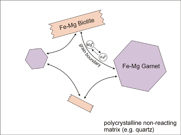
Diagram illustrating cation exchange reaction between garnet and biotite.
In order to model Fe-Mg ion exchange reaction between garnet and biotite, we made several assumptions; (1) There is no migration of grain and phase boundaries. Therefore, only exchange reaction is considered in the model, without any net-transfer reaction involving phase boundary migration. (2) Only three phases exist in our model (Figure 1); (i) Fe-Mg garnet, (ii) Fe-Mg biotite, and (iii) a non-reacting phase (e.g. quartz). The volumetrically larger non-reacting phase forms a polycrystalline aggregate with a grain boundary network. The grain boundaries become pathways for Fe-Mg diffusion. (3) Five steps or subprocesses are considered for the ion exchange reaction (Figure 2); (i) volume diffusion in garnet, (ii) volume diffusion in biotite, (iii) grain boundary diffusion, (iv) reaction (or exchange) between garnet and grain boundary, and (v) reaction (or exchange) between biotite and grain boundary. An example illustrating how these subprocesses affect concentration along grain boundaries and at points in garnet and biotite is shown in Figure 3. (4) Equilibrium compositions for garnet and biotite are obtained using temperature-dependent distribution coefficient (KD, [Ferry & Spear 1978]). The KD value during program execution is calculated using the compositions at margins (or at the portion of crystal near phase boundaries). This calculated KD is compared with the equilibrium KD of Ferry & Spear (1978). Then the chemical composition at margins is allowed to change in the direction of approaching the equilibrium KD.
Figure 2. Subprocesses for the ion exchange reaction
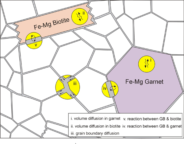
Subprocesses for the ion exchange reaction between garnet and biotite (GB: grain boundary).
Figure 3. Concentraion profiles
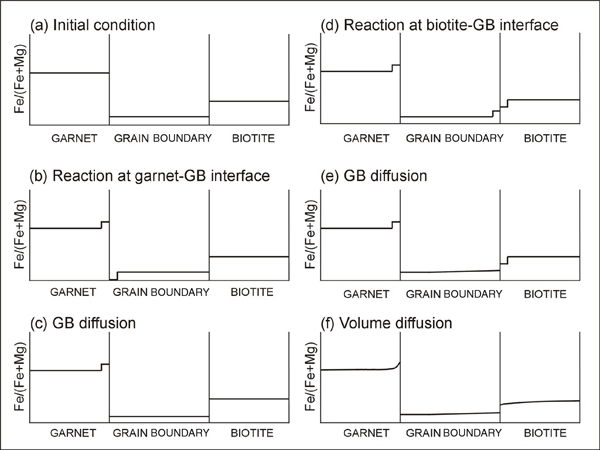
Evolution of concentraion profiles after each subprocess (GB: grain boundary).
The data model is based on two kinds of node (Figure 4). The first data structure is the "bnode" (boundary node). Bnodes are linked by segments to define grains (Figure 4a). Bnodes can have properties such as their position, link type and concentration. A bnode can be type-2 or type-3 node depending on the link type (Figure 4b). A central bnode may be connected by segments to two neighbors (type-2 node). Type-3 nodes with three segments connecting three neighbors are used to define triple junctions. The second kind of data structure is "unode" (unconnected node, Figure 4c. The unode records the material property within a volume of crystal. For our type of model where diffusive mass flux is calculated, the unodes will carry concentration information, and they can have other information such as dislocation density for other types of models. In order to allow chemical exchange between a bnode (grain boundary) and a unode (grain), special unodes are inserted adjacent to the node Figure 4d.
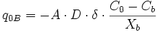
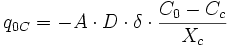
Figure 4. Data-structure of the model
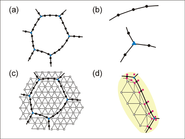
Data-structure of the model. (a) node structure for defining grains. (b) type-2node (top) and type-3 node (bottom). (c) unodes within grains. (d) special unodes at grain margins. (filled circle: type-2 node, filled triangle: type-3 node, open square: unode, filled square: special unode).
Finite-difference approximation is used for the calculation of flux and changes in concentration. For diffusion calculations at triple junctions Figure 5a, fluxes (number of atoms per unit time through an area of grain boundary section) into a type-3 node, O, from three neighboring nodes (A, B, and C) are expressed with three equations
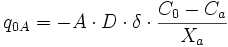
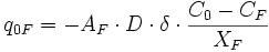
where q, A, D, C and X respectively represent flux, area of grain boundary section, diffusivity, concentration and length of a grain boundary segment (details for the quantities in the equations are shown in Figure 5a). Note that the area of grain boundary section (A) is equal to the quantity grain-boundary width (WGB) multiplied by the thickness (tsample) of the two dimensional Elle data structure, or
The total flux (Q) becomes the sum of the quantities in the above three equations, or

Then, the total flux per unit time becomes

The change in concentration per unit time becomes

divided by the volume occupied by the node O. The volume occupied by the node O can be approximated to be the half distance between node O and the considered node (A, B, or C). Thus, the volume becomes
Then, changes in concentration per time is expressed with the equation

This relation can also be applied for diffusion calculations for type-2 nodes or grain boundary segments because a grain boundary segment can be constructed by omitting one link (e.g. node C in Figure 5a) from type-3 node.
Figure 5. Diffusion calculations
Diffusion calculations (a) at grain boundaries, (b) at grain interior part. See text for detail.
For the calculation of volume diffusion in crystals, unode data structures are used (Figure 5b). Most of unodes in a crystal are evenly distributed with a two dimensional hexagonal close-packed structure, but special unodes communicating with grain boundaries are placed next to grain-boundary nodes. The evenly distributed unodes and special unodes are triangulated for the finite-difference diffusion calculation (Figure 5b). The region represented by a unode (unode O in Figure 5b) is constructed by connecting the center of gravity points of neighboring triangles. The flux into O from the neighboring regions (A, B, C, D, E and F) can be expressed with the equation:
Where q, A, D, C and X respectively represent flux, area of flux section, diffusivity, concentration and distance between two nodes Figure 5b. In a similar manner explained above, Q and aQ / a can be estimated using the flux from neighboring unodes. Then, aC / a can be estimated by dividing aQ / a with the volume occupied by unode O.
The special unodes placed adjacent to the grain boundary nodes can exchange atoms with the grain boundary nodes. The rate of exchange is assumed to be proportional to the concentration difference with a proportionality constant. The proportionality constant may have a meaning similar to the reaction constant. For the proportionality constant, we used an arbitrary value that allowed reaction sufficiently fast within a run time.
Figure 6. Parameters used for the exchange reaction
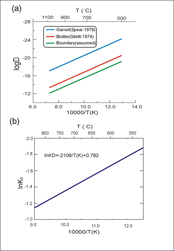
Parameters used for the exchange reaction in this study. (a) diffusivities. (b) distribution coefficient (KD) between garnet and biotite.
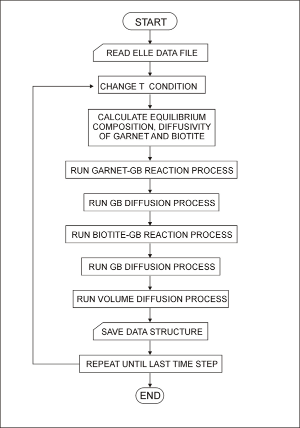
Figure 6 shows the values of diffusivity (D) and distribution coefficient (KD) used in this study. The temperature-dependent KD determines the equilibrium composition of garnet and biotite, while the diffusivity (which is also temperature-dependent) determines the rate of equilibration. The diffusivity along the grain boundary is assumed to be about one order of magnitude faster than the diffusivity within the biotite. This is based on general observations from metals [Askeland, 1994]. The overall flow chart of the model is shown in Figure 7.