Parameters in the simulations are scaled as follows: Strain is dimensionless, the height and width of the deformation box is initially 1.0, and the Poisson ratio of the triangular lattice is 0.33. The elastic constant of springs is by default 1.0. Stresses and tensile strength of springs are scaled with the elastic constant. The tensile strength of springs is by default 0.006. Grain boundary springs are weaker with respect to the default value and distributions of breaking strengths are set around the default value. In most presented simulations only the elastic constant is varied. This will produce higher or lower stresses in the model at the same strain and will thus induce fracturing at lower or higher amounts of strain. In order to relate model-parameters with real-rock values the elastic constant can be scaled, which then automatically gives real values for stress and tensile strength. Scaling-examples are given in the following paragraphs.
We performed two simulations with a competent layer that is embedded in a weaker matrix. The initial microstructure is presented in Figure 5a. The smaller grains in the centre make up the vertical competent layer. A resolution of 184800 particles is used (400x462). The elastic constant of grains in the competent layer (non-dimensional value of 1.0) is 100 times larger than that of matrix grains. The tensile strength of all grain-boundary springs is half the tensile strength of intragranular springs and has a non-dimensional value of 0.003. For this simulation the numerical parameters can be scaled to real rock values as follows. If we assume that the elastic constant of grains in the competent layer is 10 GPa (for example) then the breaking strength of grain boundary springs is 30 MPa and grains in the matrix have an elastic constant of 0.1 GPa.
Figure 5. Initial microstructures
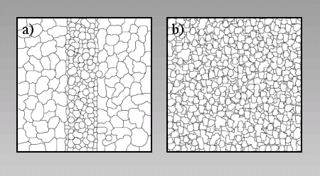
Two different initial microstructures used in the simulations. See text for further explanation.
In the first simulation the layer is extended uniaxial with incremental steps of 0.0025 percent strain (Animation 1). Colours in the animation represent differential stress where blue colours indicate low (0.0) and red colours high (0.003 times elastic constant) differential stresses (Figure 6). In the simulation the stress within the more competent layer rises because it has a larger elastic constant than the matrix. After a while a horizontal stress gradient develops within the vertical layer. Differential stresses are higher at the interface between the competent layer and the matrix than in the centre of the layer. This is an effect of the matrix-layer contact where horizontal stresses are almost zero because of the weak matrix. Geometrical irregularities at the interface of the competent layer to the matrix concentrate stresses where the competent layer is thinner. Once these stress concentrations reach the tensile strength of the springs three fractures develop almost simultaneously and break the whole layer. They show a characteristic spacing, which is found in many natural examples of fractures or joints [Price and Cosgrove 1990]. The fractures develop simultaneously in the model because the tensile strength is reached at the same time at a number of localities along the interface. Once a small fracture forms it will have even higher stress concentrations at its advancing tip because stress scales with the length of the fracture and its tip curvature [Griffith 1920; Jaeger and Cook 1979]. Therefore the fracture will cross the whole layer instantaneously because stress concentrations at its tip are beyond the tensile strength of springs and even increase during propagation (Figure 7). Fracturing will reduce the tensile stress in the competent layer and strain is localized within the fracture while it is opening. The affected area of stress release due to fracturing in the competent layer has a characteristic length-scale, which produces the regular spacing of fractures in the layer. A fourth fracture propagates across the layer shortly after the development of the three initial fractures.
Animation 1. Stiff vertical layer embedded in a weaker matrix
Stiff vertical layer embedded in a weaker matrix under layer parallel extension. Colours show differential stress where red is high and blue low stress. Mode I fractures develop in the layer and show a characteristic spacing. See main text for further explanation.
Figure 6. Stress scale for the simulations
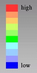
Stress scale for the simulations. Red is high differential stress and blue low differential stress. If the pressure is shown in the simulations then blue colours indicate high and red colours indicate low pressure (horizontal normal stress plus vertical normal stress components).
Figure 7. Differential stress concentrations
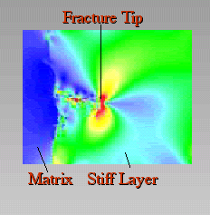
Differential stress concentrations at the tip of a fracture. The layer is extended vertically. The blue colour on the left hand side represents the weaker matrix. The fracture grows from the matrix into the stiff layer. Stress concentrations at the fracture tip drive the propagation of the fracture through the stiff layer.
The stress distribution between two neighbouring fractures has a characteristic geometry (Figure 8). Differential stresses are highest at the interface to the matrix and low in the middle of the layer and next to the existing fractures. New fractures will therefore tend to develop at the interface to the matrix and in the middle between two existing fractures. This happens towards the end of the simulation where a new fracture develops and crosses the layer so that the spacing between fractures is reduced with increasing strain. Once this secondary fracture initiates at the interface to the matrix it can propagate across the layer due to stress concentrations at its tip even if the stress in the centre of the competent layer is not tensile. In addition to the development of new fractures that reduce the spacing the four initial fractures localize strain while they open. However, opening does only effectively reduce stress if the fractures are straight. Since the initial fractures propagate mainly along grain-boundaries they show some curvature and braided geometries. These geometries hinder opening so that additional small-scale fracturing around the existing fractures is necessary in order to accommodate strain. This successive fracturing results in fluctuations of the stress in the layer throughout the animation. Once the bulk stress in the competent layer reaches the tensile strength of springs (red colour) new small-scale fractures develop and release the stress suddenly or a large fracture develops between existing fractures and reduces fracture spacing.
Figure 8. Stress distribution
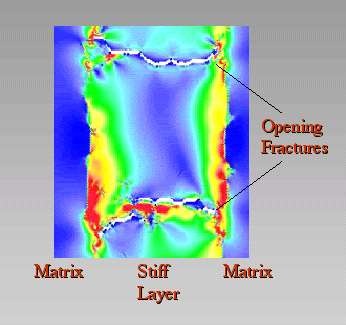
Stress distribution between two fractures in a stiff layer. Extension is vertical. The fractures are localizing strain and are opening. Differential stress is high at the interface to the matrix but low in the centre of the stiff layer. Therefore successive fractures will tend to initiate at the interface of the stiff layer to the matrix.
The second simulation shows a uniaxial compression of the same layer (Animation 2) with a strain of 0.06 percent per deformation step. The colours represent differential stress where blue indicates low (0.0) and red high (0.01 times elastic constant) differential stresses (Figure 6). The strength of the layer under compression is 3.3 times higher than its tensile strength. The initial stress pattern is similar in extension and compression with high differential stresses at the interface to the matrix and stress concentrations at irregularities. While these stress concentrations grow, small mode I tensile fractures develop in regions with highest differential stresses (Figure 9). These fractures are oriented with their long axis parallel to the maximum compressive stress. The behaviour of these mode I fractures is completely different compared to the fast propagating fractures during extension (Animation 1). Under compression stress concentration at the tips of the small mode I fractures are not high enough to support propagation. They cannot release compressive stress within the layer; they can only accommodate extension perpendicular to the shortening direction when the layer bulges.
Animation 2. Weaker matrix and layer parallel compression
Stiff vertical layer embedded in a weaker matrix and layer parallel compression. Colours show differential stress where red is high and blue low stress. Mode I fractures grow first, cluster into shear bands and lead to a transition where large scale shear fractures or faults cross the layer and induce failure. See main text for further explanation.
Figure 9. Transition between mode I and mode II fractures
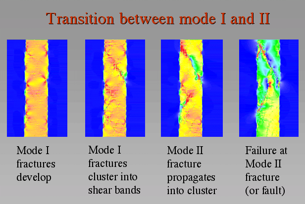
Transition between mode I and mode II fractures in a stiff layer under layer parallel compression. Stresses concentrate at geometrical irregularities on the interface of the stiff layer. Mode I fractures form in bands of compressive stresses and cluster in these bands. Later mode II type shear fractures develop out of the mode I clusters and form large-scale shear faults across the stiff layer. See main text for further explanation.
During progressive shortening of the layer regions of high stress concentrations from each side of the layer merge and form conjugate bands of high stress across the layer with an orientation of about 45° to the shortening direction. Small mode I fractures successively cluster in these bands. Finally shear or mode II fractures start to develop along the small mode I fractures within bands of high stress and propagate across the layer with an angle of less than 45° to the shortening direction. The shear fracture at the top of the layer forms a through-cutting fracture or fault along which slip takes place. The second shear fracture that develops at the lower left of the competent layer propagates towards this fault but does not merge with it and instead curves to become parallel with the fault. Both shear fractures or faults are repelling each other, which results in a distinct spacing. Close to the interface of the competent layer to the matrix sets of conjugate shears develop along the faults. Strain is mostly localized in the upper fault where significant slip takes place so that even the incompetent surrounding matrix is fractured at the fault tip.
The development of small mode I fractures, clustering of mode I fractures into bands and transition to mode II shear fractures can be theoretically predicted [Toussaint and Pride 2002] and is found in similar models [Hazzard et al. 2000] and real rock experiments [Lockner et al. 1991]. Mode II shear fractures in the second simulation (animation 2) have a different spacing than the mode I fractures in the first simulation (animation 1). Spacing of mode II fractures is narrower and seems to be influenced by the spacing of initial irregularities on the interface, which is connected to the initial grain size in the model. Mode II fractures split grains in contrast to mode I fractures that tend to develop along grain boundaries. Mode II fractures are more straight than mode I fractures since they are not opening but accommodate slip which is less efficient if they are not straight.
Two simulations were performed to investigate the development of fracture patterns in polycrystalline aggregates under pure shear deformation. The initial microstructure of the aggregates and the resolution of the models differ. The first simulation has the same initial microstructure as Animation 1 and 2 (Figure 5a), whereas the second simulation has a microstructure with smaller grains (Figure 5b). The resolution of the first simulation is 184800 particles (400x462) and the second simulation has a resolution of 737600 particles (800x922). Both simulations have distributed elastic constants for different grains and a distribution of tensile strengths of springs. The elastic constants of grains are distributed randomly and follow a Gauss distribution with a given mean m and the standard variation s. The resulting polycrystalline aggregate has a mean elastic constant of m. The tensile strength of springs is dispersed using a linear distribution with a given minimum and maximum value. Spring constants are chosen randomly within this distribution for all springs. Changing the width of the spring distribution changes the material behavior. Although the mean breaking strength will not change, the weakest springs act in a similar way to micro-flaws in the Griffith model [Griffith 1920] and concentrate stresses once they break. On a macroscopic scale this will result in a weaker strength of the material if the distribution is larger. Another effect is that material with a wider distribution of breaking strengths of springs will behave less brittle than a material with a very narrow range of breaking strengths. Once the tensile strength is reached in an aggregate with a narrow distribution failure will take place almost simultaneously throughout the whole deformation box. A wide distribution will produce initially a localization of failure at a restricted number of springs, which results in a more "ductile" behavior of the material on large scale.
The lower resolution simulation is shown in Animation 3 and Animation 4, animation 3 illustrates the fracture pattern and animation 4 the differential stress. The higher resolution simulation is shown in Animation 5 where the fracture pattern is highlighted in order to compare it with animation 3. Both simulations are performed with pure shear boundary conditions where compression is vertical and extension horizontal. The Gauss distribution for elastic constants of grains is the same for both simulations with a mean elastic constant m of 2.0 and a standard variation s of + - 0.3. The distribution of the breaking strength of springs is different for both simulations; the distribution is narrower in the first simulation and wider in the second simulation (0.0048-0.0072 and 0.0036-0.0084). The models are deformed with a stepped compressive strain of 0.06 percent and the area of the deformation box is kept constant. Colors in animation 3 and 4 show the pressure, which is the sum of the normal stress in the vertical and horizontal direction. Particles that have broken springs appear in blue.
Animation 3. Polycrystalline rock
Polycrystalline rock with a statistical distribution of grains under pure shear deformation. Colours indicate the pressure and particles with fractured springs are blue. At first mode I fractures develop and are followed by mode II shear fractures. Both show a distinct spacing. See main text for further explanation.
Animation 4. Development of the differential stress
The same simulation as animation 3 showing development of the differential stress. See main text for further explanation.
Animation 5. Large resolution simulation
Large resolution simulation similar to animation 3 but with a wider distribution in breaking strengths of springs. The evolution of structures is similar in animation 3 and 5 but animation 5 shows more dispersed development of fractures due to the wider distribution in breaking strengths.
At first the distribution of elastic constants for different grains can be seen when grains show different stress-colors. Initial fractures start to develop around grains with higher elastic constants where tensile stresses are highest. They soon start to form larger scale mode I fractures that are oriented roughly parallel to the compressive stress. Mode I fractures develop first since the tensile strength of the aggregate is less than its compressive strength. The fractures reduce the tensile stress in the horizontal direction. Three large fractures develop initially with a distinct spacing. The polycrystalline material in animation 3 has a narrower distribution of breaking thresholds than that of animation 5, so that it behaves more brittle. Animation 5 shows a material with a wider distribution of breaking thresholds and consequently behaves more ductile, fractures are more dispersed, cluster in pairs and show a spacing that is not as distinct as the spacing in animation 3.
Mode I fractures in both simulations cannot relax the compressive stress. Therefore shear fractures develop shortly after the development of the extensional fractures. These shear fractures form conjugate sets with an angle of about 35° to the compressive stress. They are propagating relatively straight in animation 3 where they cross most grains. They also tend to cross mode I fractures but sometimes merge into them. They are often repelled at the boundaries of the model. A characteristic spacing seems to exist but it is not as clear as the spacing of mode I fractures. If slip takes place along mode II fractures new small conjugate sets of shear fractures develop along the original fracture due to friction. Slip along shear fractures is the main mechanism to reduce compressive vertical stresses. Animation 5 shows a more continuous transition from mode I fracturing through hybrid shears or coupled extension and shear fracturing to pure mode II fractures. Conjugate sets of shear fractures develop at the same angle of 35° to the compression as in animation 3. The shear-fracture pattern of animation 5 is different to that of animation 3 because of a wider distribution of breaking thresholds of springs in animation 5. This produces a more dispersed localization of fractures so that these are more irregular and not as straight as the shear fractures in animation 3. However, one has to note that the finite strain in animation 5 is lower than that of animation 3 so that in animation 5 significant slip along shear fractures has not yet taken place.
Animation 4 shows the differential stress in the low-resolution simulation. The stress scale is the same as the one in the previous chapter where red represents high differential stresses and blue low differential stresses. The initial stress distribution reflects the distribution of elastic properties of grains. Once mode I fractures develop they cause stress concentrations at their advancing tips (yellow to red) and they relax stresses while they grow (blue). Once shear fractures develop they separate regions of high stress (yellow to red) from regions of low stresses (blue). In order to reduce the compressive stress significantly slip takes place along shear planes. The initial mode I fractures plus shear fractures produce columns that support the vertical load. At the end of animation 5 the column in the middle of the deformation box fails through a large scale shear fracture and the stress within the whole column is suddenly released (becomes blue). This failure is similar to the one that took place in animation 2 where a vertical competent layer was shortened. The differential stress in the whole deformation box increases upon loading, it drops shortly once mode I fractures run through the whole box, increases again and drops significantly once mode II fracturing produces failure of load supporting columns. The development and size of these columns is influenced by the initial spacing of mode I and mode II fractures.
Temperature and stress changes as well as the addition of fluid to a natural system may induce the growth of new minerals, which may include an increase in volume. This will lead to fractures in the surrounding matrix, which will enhance the permeability of a rock and influence its rheology. In this paragraph we show an example of fracture patterns that develop around several expanding grains. Animation 6 shows the fracture network and the pressure and Animation 7 the differential stress. The grains are forced to expand by increasing the radius of the intragrain particles by 0.01 percent per time step. A linear distribution is used to disperse the breaking threshold of springs and grain boundaries are weaker as described above. No deformation is applied at the boundaries of the deformation box, instead the area of the box remains constant (walls are fixed).
Animation 6. Expansion of grains
Expansion of grains that produces branching crack patterns. Animation shows fracture pattern (blue colour) and the pressure.
Animation 7. Colour scale showing the differential stress
Same as animation 6 but with a colour scale showing the differential stress. See main text for further explanation.
The fracture network that develops (Animation 6) shows no preferred orientation because no external anisotropic stress is applied. Fractures form around the expanding grains and grow in a number of directions into the matrix. They branch once they have reached a characteristic distance from the expanding grain. Fractures tend to follow grain boundaries due to lower breaking thresholds but may also cross grains. In addition to the fractures that grow from the expanding grain into the matrix grain boundaries may also fail in front of the main fracture.
The differential stress in animation 7 is highest around the expanding grains. The stress initially forms rings around the expanding grains with the highest stress at the contact between the grain and the matrix. This geometry changes once fractures develop into the surrounding matrix. Fractures separate regions of high stress values from regions of low stress values. This suggests that they are shear fractures where compressed grains (regions of high stress) slide against regions of low stress. Each time the differential stress reaches a certain value next to the expanding grain (red colour) a new set of fractures develops or fractures propagate further into the matrix in order to relax stresses again. Load supporting grains between neighbouring expanding grains start to form stress bridges.