Journal of the Virtual Explorer

Boston University's course ES301 - Structural Analysis - was just getting under way in the Spring of 2004 when NASA announced the discovery of an outcrop on Mars, at a location now called Eagle Crater. We had already planned field excursions in Massachusetts and Rhode Island but when the first Martian outcrop was displayed on the NASA Web Site (Figure 1), the addition of a "virtual" field trip to Mars became irresistible.

Using NASA's Maestro program available from http://mars.telascience.org/, in conjunction with data from http://marsrover.nasa.gov/, http://athena.cornell.edu/, and http://marsquestonline.org/, we were able to access and analyze raw images as soon as they were downloaded from the Opportunity rover. Several standard laboratory exercises and class projects were replaced by equivalent exercises using Martian data and the class morphed into an undergraduate research opportunity. Regional SettingMeridiani Planum (a.k.a. Terra Meridiani) is named for its location close to the zero-th meridian on Mars. The Eagle Crater's longitude and latitude (approximately 354° east and 2° south) places it in “a 200 to 300m section of layered rocks that are draped disconformably onto the dissected Noachian cratered terrain” [Arvidson et al. 2003]. These rocks are now thought to be water-lain sediments [Grotzinger 2004, Squyres, S.W. & Athena Team 2004, Squyres & Grotzinger 2004]. A preliminary description of the local geology and geomorphology is given in Arvidson & Athena (2004). We here concentrate on structural analysis of outcrop-scale features.

Figure 1. Panorama of Martian outcrop

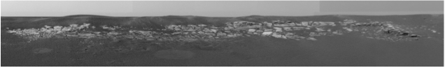
Panorama of Martian outcrop taken by Mars Exploration Rover Opportunity on Jan. 27, 2004, while it was still on its landing pad.

NASA Ref: http://photojournal.jpl.nasa.gov/catalog/PIA05158

Earth-bound structural geologists rely heavily on compass-clinometers to determine the spatial orientations of structures independent of their geographic locations. It is often more important to know that a fracture runs, say, north-south, than to know its precise location to the map to the nearest meter. Statistical analysis of such fracture orientations can yield useful information about the causal stress field, for example. Compass readings are easily corrected for the current declination of Earth's magnetic north pole to yield the direction of true north, and inclinations are estimated using a plumb-line or spirit-level. Unfortunately, these well-established techniques are not transferable to the Martian setting.

Working with data from the Opportunity rover at Eagle Crater, the first challenge was to determine the azimuths of sight-lines for photographic panoramas relative to the local Martian meridian. The current magnetic field on Mars is exceedingly weak so a compass was not on Opportunity's payload. The above-cited Web Sites displayed frequently updated photographs of the rover's sundial, however the dial changed direction as the rover moved and could not be used for independent determination of azimuth. We thus had to rely on north estimates marked on NASA's map view images or inferred from the edge directions of such images, as determined by mission engineers with access to Opportunity's guidance systems.

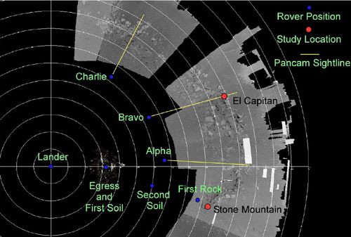
Our project base map (Figure 2a) was generated at NASA by distorting panorama photographs and "draping" them on a highly magnified aerial view of the crater taken from orbit. The crater rim is approximately 20m in diameter. The edges of the map view became our standard reference frame Figure 2b and we determined the angular range of panorama photographs by landmark recognition in conjunction with personal communications from Ray Arvidson and other mission scientists. The azimuths of the left and right edges of the panorama in Figure 1, for example, are 311° and 46° east of north, respectively, and the image spans approximately 12.5° from top to bottom. Given the distortion inherent in stitching photographic panoramas together from multiple images, these determinations are accurate only to within a couple of degrees.

Figure 2a. Outcrop distribution model

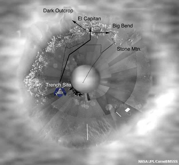
NASA's outcrop distribution model, based on a combination of rover and orbiter data, served as our base map. Locality names and rover tracks are superimposed.

Figure 2b. Mapping Eagle Crater

Mapping Eagle Crater.

The outcrop panorama was taken while Opportunity was still on its 0.5 meter-high lander (Figure 3a). The camera was mounted on a mast 1.4 meters above the lander pad [Bell et al. 2004], thus 1.9 meters above the ground, and the distance to the outcrop was about 8.0 meters. NASA estimated that the outcrop had a vertical relief of about 0.4 meters. Assuming that the lander rested on approximately level ground, we concluded that the camera's view of the outcrop must have been inclined between 10° and 15° down from the local horizontal. Later, post-egress panoramas were shot from multiple camera viewpoints and stitched together (Figure 3b). These were all approximately 4.0 meters from the crater rim but the camera was 0.5 meters closer to the ground so the inclination angles were still close to the 10° to 15° range.

Figure 3a. Sketch of Opportunity

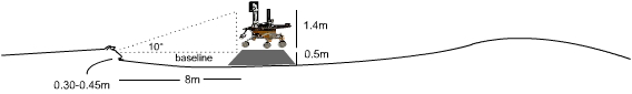
Sketch (not to scale) of Mars Exploration Rover Opportunity resting on its landing pad inside Eagle Crater. Dimensions were used to calculate the camera inclination, as discussed in the text.

Figure 3b. Location key

Key to rover locations and Pancam sightlines for detailed studies of the rim outcrop. The circles are spaced 1 meter apart.

Rotating a panorama camera's inclined sight-line about a vertical mast results in the generation of a conic surface which can be represented on a standard structural geologists' stereographic projection (Figure 4a, b). By noting sight-line azimuths and inclinations on the panorama, we were able to transfer oblique orientation data onto the stereographic net. However, it was not possible to measure the strike and dip of planar fractures or other planar structures directly from the photographs. Instead, we measured the angle of lean of a fracture's photographic trace relative to the vertical. Using a protractor, we plotted this data as a short line segment centered on the point in the stereographic projection representing the view direction for that fracture (Figure 4b).

Figure 4. Panorama photo and perspective view

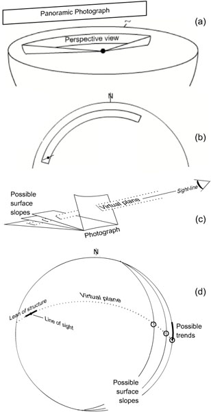
1. Panorama photo and perspective view of the conical surface swept out when an inclined camera pans. N denotes north. Small tick at left of photograph represents the trace of a plane structure such as a fracture on the photograph.

2. Lower hemi- spheric stereographic projection of the panorama. Thanks to the equal-angle property of the projection, lean may be transferred from the photograph to the stereogram using a protractor.

3. The virtual plane defined by the photographic trace and sight-line (perpendicular to the plane of the photo- graph) is here extended to intersect three possible surface slopes.

4. Stereographic projection of the geometry in (c) yields a range of possible structural trends on the ground.Panorama photo and perspective view of the conical surface swept out when an inclined camera pans. N denotes north. Small tick at left of photograph represents the trace of a plane structure such as a fracture on the photograph.

The photographic image of a planar structure only partially constrains the structure's dip. However, on a gently sloping surface, the trace is close to the plane's strike and it is useful to plot this information for a population of structures on a rose diagram, a polar plot of frequency versus azimuth. We therefore devised the following procedure to project the photograph trace back onto the map: The virtual plane defined by the photographic trace plus the camera's line of sight contains lines in a range of orientations, any one of which may be the feature's real surface trace (Figure 4c).

By plotting a great circle to represent this virtual plane, we found its intersections with a set of great circles representing possible surface slopes (Figure 4d). The unique direction that represents the structure's map trace depends on knowledge of the outcrop surface. To narrow the range of possible structural trends we studied anaglyphs of the outcrop with red/blue glasses and qualitatively categorized the 3D surface slopes as gentle, medium, and steep (We experimented with quantitative red/blue parallax measurement, but found that the human eye was adequate for our broad-brush divisions). Inherent in our method of projection data from photographs to the map is the assumption that the surface slopes towards the camera, anti-parallel to the sight-line. This is reasonable, given the rover's location close to the center of the crater, except for the area known as Big Bend. In this area, where the slope is oblique to the camera, surface morphology and coordinate triangulation were used to qualitatively constrain structural trends. For triangulation, we identified three landmarks on a photograph and then determined ternary coordinates of each end of a structural feature in one-to-one correspondence with equivalent map locations (Figure 5). As with petrologic ternary diagrams, only two of the three coordinates are independent variables.

Figure 5. Transfer of structural details

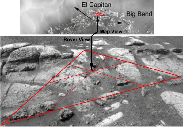
Transfer of structural details from photograph to base map using one-to-one mapping of ternary coordinates. The outcrop relief about 30-40 cm high.

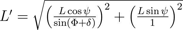
Sometimes, it is useful to estimate the lengths of linear features such as fracture traces in addition to their surface trends. This is accomplished mathematically. If L is the length of a photographic trace oriented at a lean angle of ψ relative to the photograph's vertical edge, Φ is the angle of inclination of the sight-line, and δ is the dip of the surface, which is sloping directly towards the camera, then the length L' of the trace projected onto the surface is:

Our common Earth-bound field experience leads us to visualize a straight exposure bounded by major fractures or road cuts. In contrast, Opportunity's panoramas of Eagle Crater are tightly wrapped on an approximate 10m radius. The distinction is particularly important for qualitative viewing of the outcrop. For example, parallel fractures are common in terrestrial outcrops and are often attributable to a locally rectilinear stress field. On Martian panoramas, apparently parallel fractures trending away from the viewer correspond to radial fractures on the ground. Such patterns would be highly significant in the tectonic setting of an impact crater. The rover's front and rear hazard cameras ("hazcams") present extremely wide-angle, near fish-eye views. Caution must be exercised in interpreting structures from these sources.

Earth-bound field experience also blinds us to the commonplace. For example, we learn to treat as a nuisance, or at least to ignore, the effects of weathering and erosion on surface exposures. On Mars, evidence for aeolian versus fluvial erosion is of great interest. We had to learn to pay attention to details of outcrop morphology in addition to internal structure.