Day 1
The excursion begins with a trip from Brisbane westwards to the city of Toowoomba (~700 m a.s.l). Brisbane itself is built on Palaeozoic low-grade metamorphic rocks that originated in a Devonian-Carboniferous subduction complex (equivalent to the Tablelands Complex in the southern New England Orogen). These rocks are locally overlain by Triassic and Jurassic rocks (Brisbane Tuff and Ipswich Basin). Travelling east, we encounter Mesozoic sedimentary rocks of the Clarence-Moreton Basin, before climbing onto a high plateau made of Cenozoic basalts.
Stop 1.1. Toowoomba
GPS coordinates (lat/long): -27.578959°/151.987349°
Distance from Brisbane: 125 km
The first stop is located at the eastern edge of Toowoomba and provides an excellent view to the east. The steep topography, which marks the edge of the Diving Range, is the expression of the passive margin escarpment that has retreated due to erosion. The actual escarpment in this locality is made of Cenozoic basalts that belong to the western flank of a shield volcano (Cohen, 2012). Beneath the basalts is the Mesozoic Clarence-Moreton Basin. These rocks are characterised by flat-lying clastic sedimentary successions, mostly Jurassic sandstones, siltstone, mudstones, shales and conglomerates, and some prominent coal measures. The basin started to develop in the latest Triassic and continued to subside and to accumulate sediments during the Mesozoic.
Stop 1.2. The Texas beds in Mosquito Creek
Distance from previous stop: 114 km
Travelling south from Toowoomba, we approach exposures of the Palaeozoic New England Orogen. The rocks in this area are called the Texas beds (Figure 4a) and are part of the Devonian-Carboniferous subduction complex (Tablelands Complex). Their lithology is dominated by volcaniclastic turbidites (lithic arenite and mudstone) with minor chert, limestone and mafic volcanic rocks (Donchak et al., 2007). The source of the well-bedded arenites is typically associated with silicic volcaniclastic detritus. Rocks were metamorphosed in lower greenschist facies conditions and record penetrative ductile deformation.
The area around Mosquito Creek (Figure 4b) is located in the hinge of the Texas Orocline, which is one of the most noticeable oroclinal features in eastern Australia (Figure 1c). The orocline is clearly defined by variations in the orientation of bedding and structural fabrics within the Texas beds, changing from NW-striking in the eastern limb, to NE-striking in the western limb (Figure 4a). In this locality, the dominant bedding and structural fabric is E-W (Figure 4b), as expected in the hinge zone.
Figure 4. Geology of the Texas Orocline.
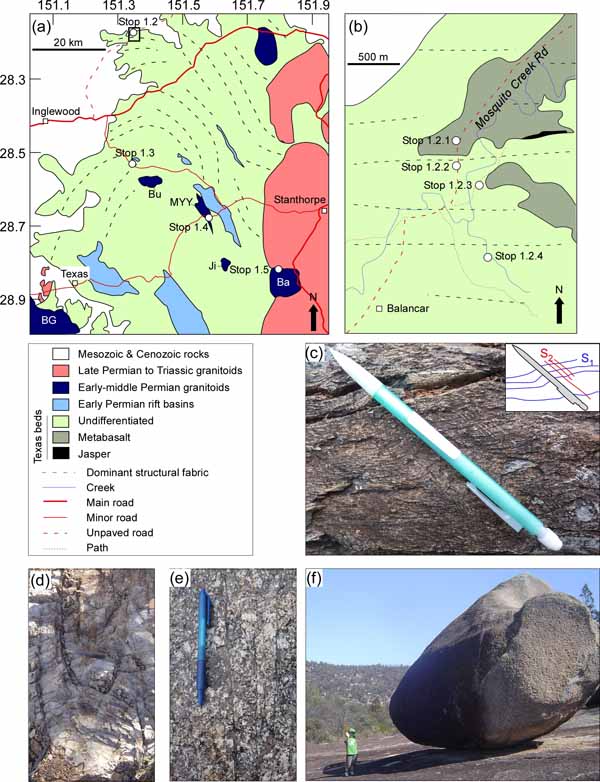
(a) Geological map of the Texas Orocline and locations of Stops 1.2 to 1.5 (modified after Li et al., 2012a). Ba, Ballandean Granite; BG, Bundarra Granite; Bu, Bullaganang Granite; Ji, Jibbinbar Granite; MYY, Mt You You Granite. Box indicates location of the inset map in Mosquito Creek. (b) Simplified geological map of the hinge of the Texas Orocline in Mosquito Creek (modified after Li and Rosenbaum, 2010) and locations of the fieldtrip sites. (c) Low strain crenulation cleavage in the Texas beds (Stop 1.2.3). (d) Isoclinal F1 fold in the Texas beds (Stop 1.3). (e) Spaced NW-SE cleavage in the early Permian Ballandean Granite (Stop 1.5). (f) A large boulder of the Stanthorpe Granite in Girraween National Park (Stop 1.6). The scale is a (very charming) 5-year-old child.
Stop 1.2.1. Metabasalt
GPS coordinates: -28.187486°/151.346113°
The rock in this locality is a greenschist facies metabasalt comprising chlorite, plagioclase and calcite. It is locally associated with pillow basalts, indicating submarine extrusive mafic volcanism, and commonly appears in association with thin-bedded layers of jasper and quartzite (Donchak et al., 2007). Spaced E-W sub-vertical cleavage can be recognised in this outcrop, parallel to the dominant structural fabric in the hinge zone of the orocline. Note that the map-scale orientations of the metabasalt bodies (NE-SW and SE-NW; Figure 4b) are oblique to the local ~E-W bedding orientation.
Stop 1.2.2. Slaty cleavage in the Texas beds
GPS coordinates: -28.189587°/151.346121°
Distance from previous stop: 0.23 km
Strong slaty cleavage is recognised in the meta-sedimentary quartz-rich beds. Rocks incorporate abundant micro-scale quartz veins, which are isoclinally folded (F1) with axial planes parallel to the dominant slaty cleavage (S1). The dominant structural fabric (S1) is consistently sub-vertical E-W.
Stop 1.2.3. Low strain crenulation cleavage
GPS coordinates: -28.191222°/151.348358°
Distance from previous stop: 0.78 km
Please note that this outcrop, as well as the next outcrop (Stop 1.2.4), are located in a private property. Entrance requires permission from the owners.
The rocks in this outcrop show overprinting relationships between the dominant S1 slaty cleavage and a later structural fabric. The latter appears as a weak crenulation cleavage (Figure 4c). Whether or not this structural fabric is directly related to the formation of the Texas Orocline is unclear. In any case, the lack of a more penetrative structural fabric parallel to the axial plane of the orocline (NNW-SSE) is somewhat surprising and may indicate that oroclinal bending involved little strain (Li et al., 2012a).
Stop 1.2.4. Pre-oroclinal quartz veins and vergence relationship
GPS coordinates: -28.197473°/151.349296°
Distance from previous stop: 0.87 km
This relatively extensive creek bed outcrop shows overprinting relationships between early N-S-trending quartz veins and the dominant E-W structural fabric (correlative to the dominant S1 slaty cleavage in Stop 1.2.2). The S1 fabric is parallel to the axial plane of minor folds and cuts the quartz veins, indicating that these veins formed prior to the development of the pre-oroclinal F1 folds. A very low angle is recognised between the orientations of the sub-vertical bedding (S0, steeply dipping to the south) and the dominant fabric (S1, steeply dipping to the north), allowing the determination of vergence relationship associated with the pre-oroclinal F1 folds.
Stop 1.3. Texas beds in Waroo
GPS coordinates: -28.535430°/151.350809°
Distance from previous stop: 59 km
Travelling south from Mosquito Creek (4a), we see occasional outcrops of the relatively monotonous succession of the Texas beds. Minor folds are not common. However, in this locality we can see meso-scale F1 isoclinal folds (Figure 4d). The NE-SW strike of the axial plane is parallel to the orientation of the western limb of the Texas Orocline. Overprinting F2 folds are not recognised.
Stop 1.4. Mt You You Granite
GPS coordinates: -28.675064°/151.581383°
Distance from previous stop: 38.5 km
The elongated NNW-SSE Mt You You Granite is located in the eastern limb of the Texas Orocline (Figure 4a) and crosses the Stanthorpe-Texas Rd in Pike Creek. Rocks are exposed in the creek bed, so accessibility is sometimes limited due to flooding.
The composition of this pluton is rather heterogeneous, varying from granite to biotite monzogranite, syenogranite and minor hornblende-biotite monzogranite. In this locality, the granite includes mafic and intermediate enclaves. A recent U-Pb SHRIMP zircon age from this locality yielded an age of 294.0±2.9 (Rosenbaum et al., 2012). This age is similar to the age of the other small early Permian plutons in the eastern limb of the Texas Orocline (Bullaganang, Mt You You, Ballandean and Jibbinbar) and is only slightly older than the ~290 Ma Bundarra Granite, which is located farther to the southwest (Figure 4a). It seems, therefore, that the Mt You You Granite is part of a belt of early Permian granitoids that is folded around the Texas Orocline.
Stop 1.5. Ballandean
GPS coordinates: -28.813810°/151.794491°
Distance from previous stop: 64.5 km
A short detour from the New England Highway will allow us to look at the Ballandean Granite (Figure 4a), which is another S-type early Permian (~295 Ma) pluton on the eastern limb of the Texas Orocline. The granite is slightly deformed and is characterised by a spaced cleavage oriented NW-SE (Figure 4e).
Visiting this area gives us an opportunity to explore some of the local wineries. This region in southeast Queensland, known as the Granite Belt, has more than 50 high-altitude (700-1200 m a.s.l) vineyards. Main wine production varieties include Chardonnay, Verdelho, Merlot, Cabernet Sauvignon and Shiraz.
Stop 1.6. Girraween
GPS coordinates: -28.833448°/ 151.935713°
Distance from previous stop: 21 km
Girraween National Park is situated in the Granite Belt immediately north of the Queensland-NSW border (Figure 3). The rocks are primarily Lower-Middle Triassic I-type granites. The largest of which is the Stanthorpe Granite, which is beautifully exposed in Girraween National Park in the form of large boulders, inselbergs and tors (Figure 4f). If time permits, it is worthwhile taking one of the short walks starting from Bald Rock Creek camping area, including the Junction (5 km return, GPS -28.830167°/151.929215°) and the Pyramid (3.4 km return, GPS -28.821884°/151.944438°).
The Stanthorpe Granite is a composite granitic suite, which together with the Ruby Creek Granite, makes the northern part of the New England Batholith (Shaw and Flood, 1981). Its composition is predominantly leucogranitic with >74% SiO2 content and <5% modal biotite content (Donchak et al., 2007). Its emplacement age is Lower Triassic (~247 Ma, Donchak et al., 2007). During the same period, magmatism occurred simultaneously along a broad (70-90 km) belt that stretched for 300 km from northeast to southwest (Figure 1b). This magmatic belt is considered to be associated with an Early-Mid Triassic Andean-type subduction zone, which was possibly subjected to asymmetric (counterclockwise) rollback in the Upper Triassic (Li et al., 2012b). Younger (230-210 Ma) granitoids are aligned along a N-S belt farther east (Figure 1b).
Following the hike in Girraween National Park, we will return to the New England Highway and continue to the Queensland – New South Wales border. The day will be concluded in the town of Tenterfield (~850 m a.s.l.), approximately ~20 km south of the state border (29 km from the last stop).