Journal of the Virtual Explorer

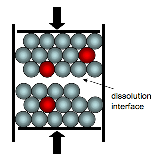
The numerical model is explained in detail in Koehn et al., 2007. It is part of the Elle Microstructure Modelling software (Jessell et al., 2001; Bons et al., 2008) and uses a lattice spring approach to calculate elastic stresses (Koehn et al., 2003; 2006; 2007). The rock is described by distinct particles (may represent actual grains) that are connected with each other via elastic springs. Particles will retain repulsive forces even if they are not directly connected. Two pieces of rock are pushed against each other with an initially horizontally aligned heterogeneity where particles can dissolve. Note that the particles can only dissolve directly at this interface. The fluid is assumed to be present at all times and diffusion is supposed to be infinitely fast. This essentially means that the model has no “real” meaningful time scale, because the process of dissolution may be diffusion limited. However the real time scale does not directly influence the roughness development (assuming that there is enough time for the roughness to develop). In the simulation the model has rigid outer walls, two frictionless sidewalls that are fixed and top and bottom walls that are being pushed inwards with a constant displacement (Fig. 3).

Figure 3. Setup of the numerical model.

[View full size]

Red particles dissolve slower.

Pinning particles are included as particles that dissolve slower. Dissolution is calculated as follows (Koehn et al., 2007)

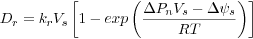
where D is the dissolution rate of the interface, k a linear rate constant that is different between “normal” and pinning particles, V the molecular volume, delta P the difference in normal stress along the interface, delta ψ the difference in Helmoltz Free Energy (sum of elastic and surface energies) between a non-stress flat and a stressed and rough interface, T the temperature and R the universal gas constant. For a derivation of the equation see Koehn et al., 2003.

In the presented simulations the following parameters were used: The Poisson ratio of the model is 0.33, the Youngs Modulus 80 GPa, the surface free energy for calcite 0.27 J/m², the molar volume for calcite 0.00004 m³/mol and the dissolution constant for calcite 0.0001 mol/(m²s) (Clark, 1966; Renard et al., 2004; Schmittbuhl et al., 2004; Koehn et al., 2007). The average normal stress on the stylolites is 40 and 10 MPa. The resolution of the simulations and the physical size vary. Figure 4 and the associated movie illustrate the growth of a stylolite in a high-resolution simulation with 184,000 particles (400 in the x direction).

Simulation 4. Teeth development in a high-resolution simulation (400 grains in x direction).

View simulation

Real physical length of the stylolite is 2m and the average normal stress 10 MPa.

Figure 4 and the associated movie already illustrate the rich dynamics of the roughness growth. In the beginning the interface is fluctuating and teeth are not growing very fast. Once the interface reaches a critical wavelength the growth mode changes and larger teeth develop relatively fast. The teeth are still fluctuating on the smaller scale and may be destroyed from the top or bottom but are relatively stable compared to earlier fluctuations of the roughness. The following section will discuss these different growth modes in detail.