Appendix A. The influence of uppermost crustal composition in the inversion process and obtained VS structure.
The realistic modeling of uppermost crustal structure is very important in the non-linear inversion of the dispersion data and influences the obtained structures at mantle depths. One example is the inversion in cell b-1, in the Corsica offshore. The same dispersion data are used (phase velocities available in the period range 20 – 80 s and group velocities for 10 – 150 s with relevant single point errors) in two cases of the inversion. Since the smallest period is 10 seconds, the uppermost crust is not well resolved and its structure should be fixed using independent information. Two different parameterization of the uppermost crust (Table 2) are used and the obtained two sets of solutions have significant differences also in the mantle structure. Listed in Table 2 are values of VP, VS, thickness and density in the first five uppermost crustal layers that are kept fixed in the inversion. The following 5 layers are parameterized in both cases using five parameters for layer thicknesses, five parameters for VS and one parameter for VP/VS ratio. The used parameterization in both cases (central values, steps, ranges) is listed in Table 3. The explored parameter space (grey area in Fig. 23) is similar in both cases.
Table 2. Parameterization of the uppermost crust
layer |
I case | II case | ||||||
|---|---|---|---|---|---|---|---|---|
| h (km) | Vs (km/s) | Vp (km/s) | ρ (kg/cm3) | h (km) | Vs (km/s) | Vp (km/s) | ρ (kg/cm3) | |
| 1 | 0.06 | 0.00 | 1.50 | 1.03 | 0.06 | 0.00 | 1.50 | 1.03 |
| 2 | 2.94 | 1.20 | 2.25 | 2.10 | 1.44 | 1.20 | 2.10 | 2.10 |
| 3 | 0.50 | 1.50 | 2.60 | 2.20 | 0.03 | 1.35 | 2.35 | 2.20 |
| 4 | 1.30 | 3.85 | 6.66 | 2.60 | 1.00 | 2.80 | 4.80 | 2.45 |
| 5 | 1.20 | 3.95 | 6.84 | 2.80 | 1.00 | 3.00 | 5.20 | 2.55 |
Table 3. Central values, steps, ranges
parameters |
I case | II case | ||||||
|---|---|---|---|---|---|---|---|---|
| Vp/Vs | Vp/Vs | |||||||
| P0 | 1.73 | 1.73 | ||||||
| H0 (km) | step (km) | Hmin | Hmax | H0 (km) | step (km) | Hmin | Hmax | |
| P1 | 12.0 | 4.0 | 4.0 | 16.0 | 14.0 | 4.0 | 10.0 | 22.0 |
| P2 | 4.0 | 4.0 | 4.0 | 12.0 | 22.0 | 8.0 | 14.0 | 38.0 |
| P3 | 40.0 | 20.0 | 20.0 | 60.0 | 40.0 | 15.0 | 25.0 | 55.0 |
| P4 | 45.0 | 45.0 | 45.0 | 90.0 | 70.0 | 30.0 | 40.0 | 100.0 |
| P5 | 135.0 | 45.0 | 45.0 | 180.0 | 120.0 | 50.0 | 70.0 | 120.0 |
| VS0 (km/s) | step (km/s) | VSmin | VSmax | VS0 (km/s) | step (km/s) | VSmin | VSmax | |
| P6 | 4.50 | 0.25 | 2.25 | 4.75 | 3.60 | 0.15 | 2.25 | 4.30 |
| P7 | 3.35 | 0.15 | 3.20 | 4.95 | 4.20 | 0.20 | 3.60 | 4.80 |
| P8 | 4.30 | 0.15 | 3.70 | 4.75 | 4.30 | 0.15 | 3.85 | 4.90 |
| P9 | 4.00 | 0.20 | 3.80 | 5.00 | 4.40 | 0.20 | 4.00 | 4.80 |
| P10 | 4.35 | 0.15 | 3.60 | 5.10 | 4.30 | 0.30 | 4.00 | 4.90 |
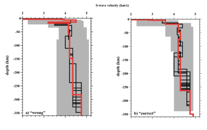
Figure 23. Inversion results for cell b-1.

Non-linear inversion results for I case (a) and II case (b) of the uppermost fixed crust. VS models that are solution of the inverse problem are shown with thin black lines and the selected cellular model is represented by thick red line. The grey areas delimit the explored parameter’s space sampled by the simultaneous non-linear inversion of phase and group velocity of Rayleigh waves.
The obtained two sets of solutions are different not only in the shallow crustal structure but also at mantle depths (Fig. 23). In the first case the uppermost fixed crust is defined as the oceanic-like with layer of water, two sedimentary layers and two high-velocity layers (Tab. 4). In the case of the offshore of Corsica this is not realistic and the uppermost crust can be defined as “wrong”. The obtained set of solutions for this case is shown in Fig. 23a. All accepted models have a high-velocity layer (VS about 4.25-4.50 km/s) at depths of about 5-15 km. This layer is followed by thin, low-velocity layer ( VS about 3.2 km/s). The velocity in the mantle increases slightly with depth below 20 km. The representative solution selected by LSO (processing all cells of the study area) is presented by thick line in Fig 23a. It is characterized by high VS (about 4.50 km/s) at depths of 5 to 15 km, followed by thin low velocity layer. Below 20 km of depth VS increases from 4.15 to 4.75 km/s at about 280 km of depth. More realistic uppermost fixed crust is used in the second case of parameterization: water layer is the same and it is followed by sedimentary layers with increasing velocities and densities and upper crustal layer with VP of 5.20 km/s. The obtained set of solutions (Fig. 23b) is consistent with the known geodynamical setting of the region and it is characterized by crustal layer with VS of 3.45-3.60 km/s reaching depth of about 20 km. This layer is followed by mantle with VS between 4.15 and 4.40 km/s and low-velocity layer with VS about 4.00 – 4.20 km/s. The deeper mantle layer has VS about 4.60 - 4.75 km/s and starts between 200 and 250 km of depth. The selected representative solution (thick line in Fig. 23b) has a crust about 20 km thick, a mantle lid about 50 km thick, a LVZ with VS of 4.20 – 4.30 km/s located between 70 and 270 km of depth. The following layer has VS about 4.75 km/s. This model is fairly consistent with the geological interpretation of the obtained VS models along the section shown in Fig. 22 (see section “Discussion” for details).
The realistic modeling of the crustal layers especially at shallow depth has a very important role in the inversion process and is crucial for the realistic modeling of the upper mantle. The usage of “standard” crust in the inversion of tomographic data biases the results of the inversion also at depths below 100 km, especially in the regions with very complex structure as the study region.