Data and Methodology
Seismograms recorded at ten sites located on the four south Indian granulite terranes and neighboring Archean Dharwar craton were analyzed to determine the crustal shear-wave structure of these exhumed high-grade terranes (Fig. 1). These seismographs were installed and operated by the National Geophysical Research Institute, the Indian Institute of Astrophysics, the India Meteorological Department, Andhra University and the University of Cambridge, UK. The Visakhapatnam (VIZ) seismic station was located on the Eastern Ghat Granulites, Kodaikanal (KOD) on the highland massif of Madurai Granulites, Trivandrum (TRV) on Kerala Khondalites, Mettuppalayam (MTP) and Madras (MDR) on the Nilgiri-Madras Granulites and Pichi (PCH) close to the Noyil-Kaveri boundary that separates it from the Madurai block. Three additional sites at Mysore (MYS), Gundulpet (GDP) and Gorur (GRR) were located north of the orthopyroxene isograde that separates the granulites from the granite-greenstone terranes of western Dharwars, although dominant rock types in the vicinity of MYS and GDP are of high-grade amphibolites/granulite facies. Between them, these seismograph stations cover most of the major blocks of the Indian shield granulites and thus provide an opportunity to make a comparative study of their crustal cross-sections.
Figure 2. Receiver Functions
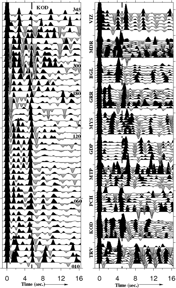
Receiver functions for KOD, plotted as a function of azimuth (left panel). Moho converted Ps phase can be identified at ~5.15±0.02 s. RFs’ for other stations are shown on right panel.
Receiver Functions, Crustal Thickness and Vp/Vs value
Determination of crustal structure beneath a single seismic station using receiver functions is now a well-established seismological technique. We used the P-wave receiver function technique (Langston, 1979, Ammon, 1991) to extract the P-to-S converted phases generated at various sub-surface seismic discontinuities. In the present study, we use time-domain iterative deconvolution technique developed by Liggoria and Ammon (1999) to extract the Ps converted phases. This method, recognizing that the radial seismogram is a convolution of the vertical component with the earth structure, proceeds to extract the impulse function by designing a time series which when convolved with the vertical component, would approximate the horizontal component. This is accomplished by a least-squares minimization of the difference between the observed horizontal seismogram and a predicted signal generated by the convolution of an iteratively updated spike train with the vertical. This procedure renders the resulting receiver functions relatively free from any deconvolution-induced noise such as those observed in the water-level deconvolution technique.
Receiver functions were calculated for all high signal-to-noise ratio seismograms of events with magnitudes greater than 5.5 lying within the epicentral distance range of ~30° and 90°, after ascertaining that they were free from polarization anomalies (Kanasewich, 1975, Jurkevics, 1988). We low-pass filtered these receiver functions by smoothing with a Gaussian of 3.5, thereby eliminating frequencies greater than ~1.7 Hz. Fig. 2 shows the radial component of receiver function for all the seismic stations.
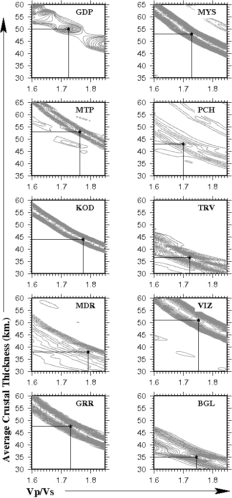
We used the H-σ stacking procedure to determine the thickness (H) and the average Vp/Vs value of the crust beneath the seismograph site (Zandt et al. 1995, Zhu and Kanamori, 2000). In this technique, the weighted sum of the receiver function phases (Ps, PpPms and PpSms + PsPms), stack to a maximum for the correct combination of H and Vp/Vs value.
The Vp/Vs and the crustal thickness thus determined provide a first-order estimate of the Moho depth beneath a seismic station, and the petrological character of the crust in term of its Vp/Vs value (or Poisson's ratio) (Christensen 1996). Fig. 3. show the crustal thickness and Vp/Vs value thus determined for each of the seismic station.
Crustal Shear-wave Structure
Receiver functions are more sensitive to the impedance contrast across an interface than the absolute shear-wave speed of the layers. Therefore, analysis and interpretation of converted phases alone suffer from a trade-off between the layer thickness and the average S-wave velocity (Ammon et al. 1990). Surface wave dispersion data, on the other hand, are more sensitive to average shear wave velocity at various depth ranges than to their gradients. Joint inverse modeling of both receiver function and surface-wave dispersion data, thus constrain models of the earth structure more tightly than either of these data analyzed separately. Therefore, we inverted P-wave receiver functions jointly with surface wave group velocity data (Julia et al. 2000, Hermann, 2004). The method expresses the least squares problem in terms of eigenvalues and eigenvectors extracted by using Singular Value decomposition to estimate a crustal model parameterized by shear wave velocity in a crust consisting of a stack of thin layers.
The analysis also yields the respective covariance and resolution matrices to evaluate the quality of the solution. Surface wave dispersion data were taken from (Mitra et al. 2006).
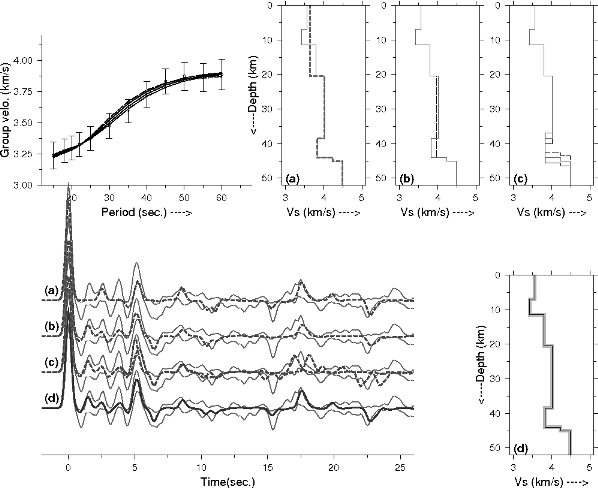
Figure 4. Crustal shear-wave velocity structure at KOD
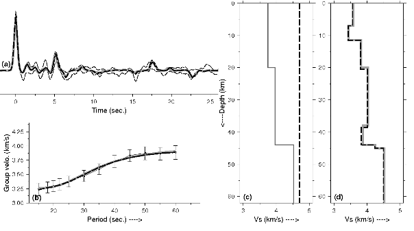
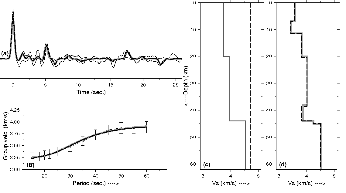
Crustal shear-wave velocity structure at KOD derived by jointly inverting the stacked radial receiver function (a) and surface-wave data (b). Two starting models (a half-space model with shear-wave velocity of 4.7 km/s. and a two-layer model) selected for inversions are shown in (c). The final inverted crustal models are shown in (d) along with observed and synthetic receiver function and surface-wave group velocity (a,b).
To enhance the signal-to-noise ratio, receiver functions for events lying in small bins of 5° x 5° back-azimuth and epicentral distance were stacked and their ±1σ standard deviation bounds calculated. The input velocity model chosen for initiating the inversion process was a stack of 1.0 to 1.5 km thick layers with half-space velocity of 4.7km/s (Fig. 4c). A homogeneous half-apace model introduces minimum a priori information in the inversion process and reduces the possibility of bias creeping into the inverted models. The shear-wave velocity model evolves freely from the half-space model, minimizing the misfit of the two data sets to an optimum level, and exploring the whole range of model space. In the next step of the inversion process, layers with closely similar shear-wave velocity were clubbed together to evolve the next, more simplified, starting model for inversion. This was iteratively repeated till a satisfactory solution was attained that simultaneously provided an optimally good fit to both the receiver function as well as the surface-wave dispersion data (Fig 4a,b).
To examine the dependence of final model on starting model, we inverted the data with another model developed by forward modeling of the primary phases of receiver function and surface-wave data (Fig. 4c, two-layer model, gray line). However, we do not see significant change in the final shear-wave velocity model obtained by joint inversion, starting with these two different models (Fig. 4d). Finally, we also tested the main features of the model obtained by inversion through forward modeling of the receiver function and surface-wave dispersion data (Fig. 5).
The upper and lower crustal layers were smoothed (Fig. 5a,b), depths of the Moho discontinuity was shifted up and down (Fig. 5c), and their effect was observed on the final fit. Minor features which do not significantly distort the fit were removed, and only those were retained which were necessary for an optimum fit between the data and synthetics. The final velocity model thus obtained for KOD (Fig. 5d) can be described as a two-layer crust consisting of an upper layer of 20 km thickness and an average Vs=3.59 km/s, underlain by a 23.5 km thick lower crust with Vs=3.99 km/s. Additionally, the KOD data requires a Moho at 43.5 km and a lower velocity layer in the upper crust (7-11.5 km, Vs=3.39 km/s.) for an optimal fit of the synthetics to the observed RFs'. These are the most robust features of the velocity image beneath KOD. Seismic structure of other granulite stations is described in the following section.
Figure 5. Test results for significance of main crustal features
(a) smoothing upper crustal features, (b) smoothing lower crustal features, and (c) moving the moho up or down by 1.5 km. Smoothing degrades the fit of synthetics and real data as shown in corresponding figures. For exp. changing the moho depth, disturbs the fits of phases at 17.5 and 22.5 s., (d) final shear-wave velocity structure.
The Granulite Terranes of the Indian Shield
Seismic characteristics (crustal thickness, Vp/Vs value and subsurface shear-wave velocity structure) of the crust beneath other stations located on the south Indian high-grade terranes were determined in the same fashion as described above for KOD. Receiver functions for all sites are plotted in Fig. 2. Receiver functions for the granulite (TRV, KOD, PCH, MTP, MDR, VIZ) and western Dharwar (GDP, MYS, GRR) stations are complex compared to those observed for the eastern Dharwar Craton (BGL) included here for comparison. Most of the radial receiver functions, particularly those from TRV, KOD, MTP, MYS, GRR, and VIZ, show significantly coherent intra-crustal P-to-S converted phases arriving between the direct P- and the Moho-converted Ps phase, indicating a multi-layered seismic structure. Vp/Vs values and crustal thickness for each of these stations were determined using the method described earlier for KOD, and these are summarized in Figures 3, 7 and Table 1. These results indicate a substantially thicker crust (~8 km) beneath the western Dharwar and the granulite terranes than those observed for Archean eastern Dharwar Craton (Rai et al. 2003). Some of the granulite terrane stations like KOD, MDR, MTP show relatively higher Poisson's ratio (Vp/Vs greater than 1.75) indicating a more mafic lower crust underneath (Rudnick and Fountain, 1995, Chevrot and van-der Hilst, 2000). A more mafic lower crust has also been inferred from fluid inclusion studies which are well documented in the geological literature of granulites (Friend and Nutman, 1992, Bartlett et al. 1995, Mohan et al. 1996, Bhattacharya & Sen, 1996, Ray et al. 2003). Exceptions to this general observation are a thinner crust at MDR (~38 km) on the eastern edge of the Nilgiri Granulites, and TRV (~36.5 km) located on KKB and relatively lower Vp/Vs (~1.70) at PCH.
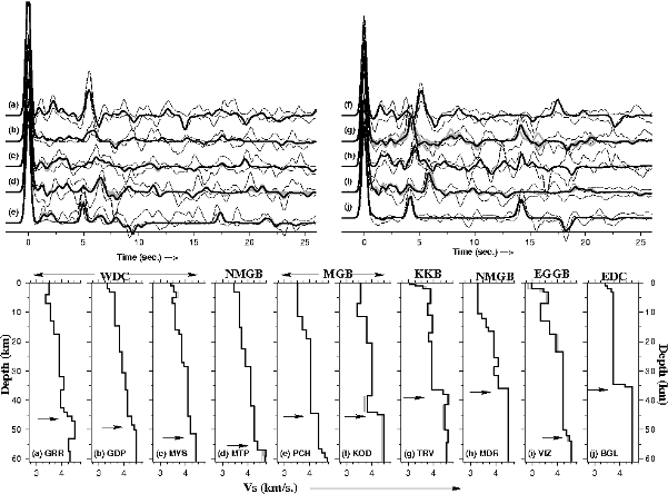
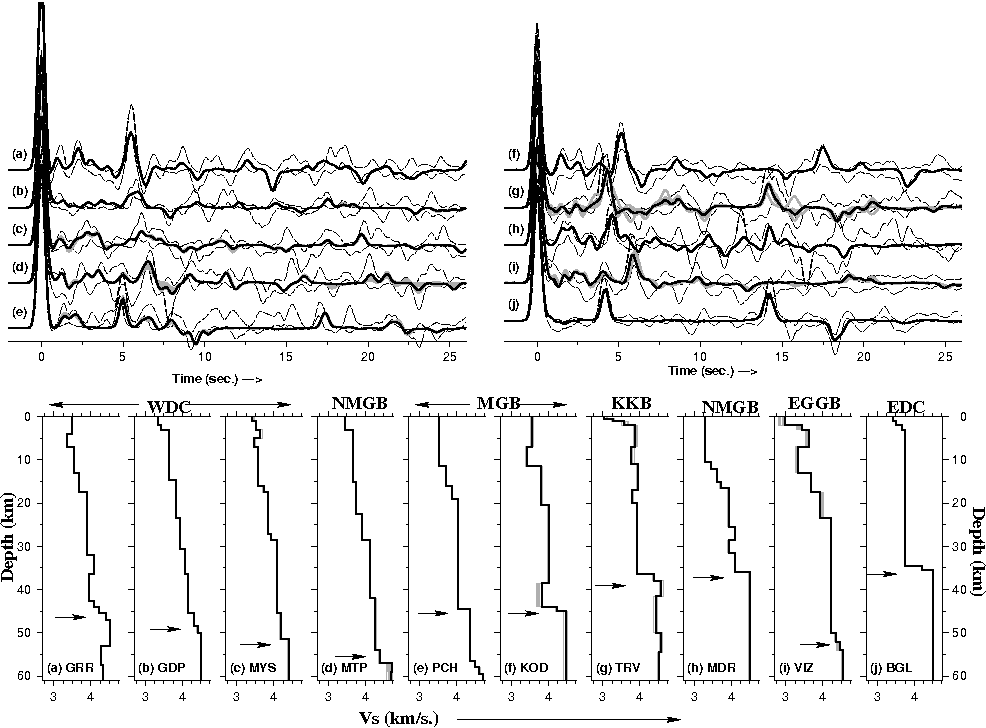
Figure 6. Seismic velocity structure
Seismic velocity structure beneath various stations, located on different terranes of the Indian shield. Dashed lines in receiver function plots denote the ±1σ bounds of the stacked receiver functions; solid lines denote the synthetic receiver functions corresponding to shear-wave velocity structure shown at the bottom.
High quality radial receiver functions for these stations from narrow bins of back-azimuths and epicentral distance ranges were stacked to enhance the signal-to-noise ratio and inverted jointly with the respective surface wave data as was done for KOD. The inversion results summarized in Fig. 6 show that the internal structure of the crust of the western Dharwar Craton and of the Granulite terranes is more complex compared to that of the eastern Dharwar, and has a transitional Moho in contrast to the rather sharp Moho beneath the eastern Dharwar. Moreover, the western Dharwar crust is substantially thicker than the eastern Dharwar crust and increases in both complexity and depth southward as one approaches the highly diffused granite-granulite boundary (GDP, MYS in Fig. 6 b,c) and crosses into the adjoining Nilgiri Granulites (MTP in Fig. 6d). Further south, the PCH crust (Fig. 6e), generally considered to be a part of the Nilgiri Granulites, also has a multi-layered structure with a gradational upper crust and a relatively sharp Moho similar to that of KOD (Fig. 6f) in the Madurai Granulites, crustal thickness is also same (~43km). However, it has a lower Vp/Vs value (~1.70) requiring a higher fraction of felsic components possibly created by stacking of two upper crusts. The two remaining granulite sites, TRV and VIZ, lie respectively on the southwestern Khondalite (meta-sedimentary granulites) terrane, and the Eastern Ghat Granulites. TRV (Fig. 6g) shows a relatively thinner crust (36.5 km), and Vp/Vs value of 1.72, typical of granulites (Rudnick & Fountain, 1995). In contrast to this, VIZ (Fig. 6i) has a substantially thicker crust (~51 km) like the western Dharwar, a complicated upper crust and a gradational transition to mantle velocities. It is interesting to compare the nature of the lower crust in the western Dharwar and the granulite terranes with the eastern Dharwar. The average lower crust Vs in Eastern Dharwar (station: BGL) is ~3.70 km/s. In contrast, the lower crust Vs at all other stations vary between 3.85-4.15 km/s suggestive of relatively more mafic composition. The upper crust (up to 15 km depth) average velocity for the Western Dharwar and Granulite terrain stations is ~3.65±0.1 km/s.
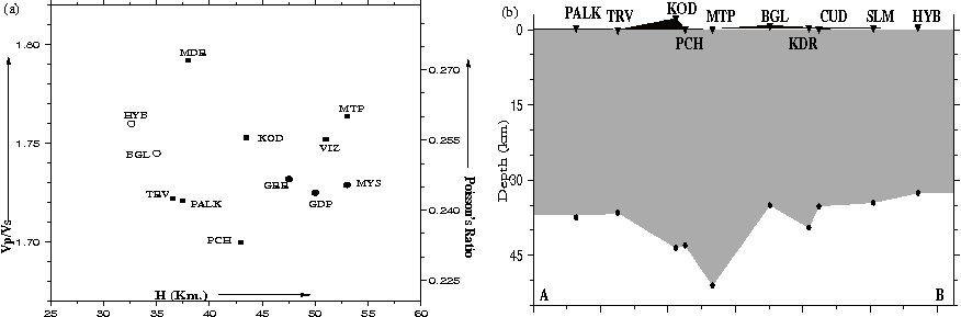
Figure 7. Crustal Thickness

(a) Crustal thickness versus Vp/Vs (Poisson’s ratio) beneath various seismic stations in the south Indian shield. Stations on eastern Dharwar (HYB, BGL) are shown by open circles, those on Western Dharwar (GRR, GDP and MYS) are shown by filled circles and Granulite terrane stations are shown by filled squares (some of the values is taken from Gupta et al. 2003 and Rai et al. 2009). (b) Variation of crustal thickness along traverse AB (Fig. 1).
Table 1. Broad-band station locations and crustal parameters derived in this study
| Station | Location | Lat. (Deg.) | Long. (Deg.) | Elev. (m.) | H (Km.) | Vp/Vs |
|---|---|---|---|---|---|---|
| TRV | Kerala Khondalites | 8.51 | 76.96 | 10 | 36.5±0.9 | 1.722±0.017 |
| KOD | Madurai Granulites | 10.23 | 77.46 | 2258 | 43.5±0.7 | 1.753±0.015 |
| PCH | Nilgiri Granulites | 10.51 | 76.35 | 142 | 43.0±2.0 | 1.700±0.016 |
| MTP | Northern Granulites | 11.32 | 76.94 | 227 | 53.0±1.1 | 1.764±0.030 |
| MYS | Northern Granulites | 12.31 | 76.62 | 698 | 53.0±2.4 | 1.729±0.030 |
| MDR | Nilgiri-Madras Granulites | 13.07 | 80.25 | 10 | 38.0±1.1 | 1.792±0.041 |
| VIZ | Eastern Ghat Granulites | 17.72 | 83.33 | 3 | 51.0±2.5 | 1.752±0.040 |
| BGL | Eastern Dharwar Craton | 13.02 | 77.57 | 843 | 35.0±1.3 | 1.745±0.020 |
| GDP | Western Dharwar Craton | 11.79 | 76.65 | 761 | 50.0±0.4 | 1.725±0.011 |
| GRR | Western Dharwar Craton | 12.82 | 76.06 | 792 | 47.5±0.8 | 1.732±0.010 |