Fitting of a focal mechanism to the first arrival data is performed in the shockwave flash (.swf) file called "FirstMo.swf." This is a flash movie with three frames. The first frame initializes variables and defines actionscript functions that handle the controls at the top of the window. The second frame loads the XML data, parses the tags, and projects the data. The third frame directs the movie to return to the second frame. In this way, the flash movie monitors the external data file and responds to changes whenever they are saved.
Figure 4. Example
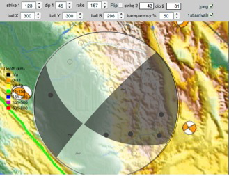
The background image may be a geological map showing the epicenter location, for example.
With the xml data in place, the user can locate and resize the focal mechanism beach ball, varying the strike and dip of one nodal plane and the rake of the intersection with the second nodal plane. The resultant strike and dip of the second nodal plane are output (they cannot be independently altered because of the constraint of orthogonality). Pseudo-code to maintain nodal plane orthogonality is illustrated in Example 3. Black and white quadrants can be interchanged using the "flip" button and the default black color can be changed using the standard USGS color table for shallow, intermediate, and deep earthquakes.
Example 3. Pseudo-code to maintain nodal plane orthogonality
x = SIN(rake) * COS(dip1) * COS(strike1) – COS(rake) * SIN(strike1);
y  = – SIN(rake) * COS(dip1) * SIN(strike1) – COS(rake) * COS(strike1);
trend = ATAN (x / y);
plunge = ACOS(SQRT(x ^2 + y ^2));
strike2 = trend – 3 * pi / 2 modulo 2 * pi;
dip2 = pi / 2 – plunge;