Journal of the Virtual Explorer

In this simulation (Simulation 1a) relative solid-solid to solid-liquid surface energy ratios are such that the wetting angle is 10° at equilibrium. The melt fraction is fixed at 2%. The starting microstructure already shows some disequilibrium features, so that not all melt pockets have wetting angles of exactly 10°. However during the simulation grains quickly adjust to an equilibrium shape (convex triangle, E-shape) that is relatively stable. This behavior was predicted by Laporte et al. (1997) for wetting angles in a static system that are lower than 60° when grains have similar sizes.

However, continuous grain growth due to a reduction of the overall surface energy of the aggregate is disturbing the equilibrium wetting angles. This becomes obvious when small grains collapse completely.When the grains reach a certain critical size the total energy of their surfaces is relatively high because they have a very high surface curvature. Therefore they will dissolve or melt with an increasing velocity. Decreasing their size will just increase the surface curvature so that they will collapse completely in a relatively short time (relative to grain boundary movements of the other grains). During the collapse melt pockets are distorted and surrounding grains are bulging towards the disappearing grain until they are disconnected. The final collapse of the small grain leaves relatively large melt pockets (disequilibrium shape, D-shape). These disequilibrium structures disappear slowly (relative to their appearance) while the surrounding grains adjust their shape. Finally, melt pockets reappear that show the equilibrium shape and corresponding wetting angles.

The transition from an E-shaped to a D-shaped melt pocket increases its area and therewith its ratio of area to perimeter, forcing melt to be redistributed from other melt pockets into the D-shaped melt pocket. In Figure 3 the ratio of area vs. perimeter is shown for a single, D-shaped melt pocket and its changes over time during the simulation. Once the surrounding grains collapse, the D-shaped melt pocket splits into two convex triangles and the excess melt is redistributed to other E-shaped melt pockets.

Figure 3. Pictures of different stages during simulation 1a

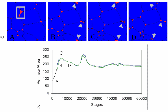
1. Pictures of different stages during simulation 1a. Location of observed D-shaped melt pocket in b) is outlined with gray square.

2. During the simulation, the are and the perimeter of the different melt pockets is calculated. The ratio of area to perimeter shown here corresponds to the melt pocket outlined in a) during the simulation. The initially black curve corresponds to the D-shaped melt pocket (located in A). In picture B, the initially E-shaped melt pocket split into two E-shaped melt pockets, the blue and green curves correspond to these E-shaped melt pockets. The peaks of the curves at 7000, 23000 and 45000 stages developed during the simulation at points where the formation or destruction of D-shaped melt pockets (see arrows in a) require the redistribution of melt.

The wetting angles of the melt pockets was initially set to 10°, but ranges between different values during the simulation. Especially during the formation of D-shaped melt pockets and the accompanying redistribution of melt, the E-shaped melt pockets display pronounced changes of their wetting angles. After destruction of the D-shaped melt pocket and accompanying redistribution of melt into the E-shaped melt pockets, the wetting angles tend to adjust again to 10°. This is in contrast to what was predicted from e.g. Laporteet al. (1997). It appears that the wetting angle cannot be treated as a constant parameter in short time periods. This also implies that the mean curvature of solid-liquid interfaces is not constant as was suggested by Laporte etal. (1997).

If the melt fraction is not fixed but allowed to grow, the melt pockets simply grow in size until no more solid grains exist. If the melt fraction is limited to a certain percentage, the melt pockets grow (or shrink) until the desired percentage is reached. The amount of melt introduced into the simulation has no influence on grain shape, noron the rate of development of the melt pockets (with the exception of unlimited melt where all the grains disappear).

In simulation 1b the melt pockets are surrounded by three regularly shaped grains so that the grains have an almost perfectly round shape. The melt pockets are distributed within the gussets of the grains. This simulates the grains having isotropic surface energies that are already minimized at the start of the simulation. The wetting angle is set to 10° and the melt fraction is fixed to the starting value. Since the surface energies of the grains is already minimal at the beginning of the simulation, no adjustment of the surface energies and therewith no change of shape of the crystals is necessary. Only where small distortions of the round grains occur (e.g. at the bottom of the simulation, because of the wrapping boundaries), the grains collapse and the melt pockets form a D-shape. Eventually this would continue throughout the whole area of the simulation since the distortions would work their way upward. However, it is clear that rounded (or spherical)shapes of the grains results in very little change of shapes of the melt pockets and surrounding grains and a very stable aggregate.

In simulation 2 and 3, the relative solid-solid to solid-liquid surface energies are set such that the wetting angle is 60° at equilibrium. The melt fraction is static at ~2%. The duration of the run is shorter than in the first simulation since equilibrium is reached much earlier. The boundaries of the E-shaped melt pockets straighten due to the higher wetting angle.A quick distribution of the melt into pockets at grain corners is observed and was predicted by [Bulau et al. (1979)].

Simulation 3 of a wetting angle of 120° showed the predicted results of [Bulau et al. (1979)]. At high wetting angles, the equilibrium shape of melt pockets is rectangular and all the triangular shaped melt pockets disappear with their melt being redistributed into the rectangular shaped melt pockets. This behavior is completely due to the high wetting angle.

In addition to the simulations described above, different parameters for the mobility of the respective boundaries were used in a set of simulations to analyze the influence of this parameter. The simulations show that variations of the mobility of the boundaries influences the velocity of the boundary-movement but have no impact on the resulting grain fabric or the equilibrium geometry of the melt pockets. All the simulations use the same starting grain fabric, surface energies and duration of simulation.The mobility of the boundaries was set to the highest (lowest) possible values or are equal. The movies shown below all have 25 frames per second so changes in the velocity of boundary movement are solely a result of the variations in the boundary mobility.

In simulation 4, the mobility of the boundaries was set to be equal at 10^-11, in simulation 5 the mobility of the boundaries here was set to be equal at 1^-10 and in simulation 6 the mobility of boundaries here was set to 1^-10 for the ss boundaries and 1^-11 for the sl boundaries.