Data and Method
To accurately model and simulate different deformation scenarios, reconstruction software has to be able accommodate such tectonic scenarios, and in a way that allows quantitative paramterisation. Thus the Pplates software (Smith et al. 2007) was designed to allow structural geology and tectonics research concerned with the effects of heterogeneous deformation and faulting, from regional through to planetary scales. As described within Smith et al. (2007), the Pplates software does this by allowing the use of deformable and tearable meshes (irregularly tessellated polyhedrons) involving triangular mesh faces. Nodes are connected using a Delaunay algorithm and correspond to a mesh surface represented in three dimensions to conform to the surface of the Earth (Smith et al. 2007).
Motion data can be imposed on individual nodes while the node-connecting springs can be kept rigid or be used to distribute stress and strain among the mesh faces. If a point of latitude and longitude within the interior of a mesh face is moved, the equivalent Cartesian coordinates are calculated and expressed as a vector (Smith et al. 2007). The addition of this vector and the rotation matrix gives a new vector of Cartesian coordinates that are used to provide the new latitude, longitude, and altitude of the moved point. A transformation matrix, calculated using the three initial and final Cartesian vectors, provides the movement and deformation of the individual mesh face. The transform matrix replaces the Euler rotation matrix whenever points associated to a deforming mesh face are moved (Smith et al. 2007). Deformation on any mesh face can thus be applied to any data carried by the mesh, for instance in this reconstruction of the Andean Margin the meshes carry the NOAA ETOPO2 data in order to allow variations in crustal thickness implied by mesh deformation to be monitored.
To constrain mesh deformation we predominately utilised geological data provided by balanced cross sections (Figure 2). Such shortening data, and associated geological data present in the referenced sources, provide one constraint as to the timing and degree of deformation occurring during the formation of the Patagonian and Bolivian Oroclines. A lack of published data exists regarding the specific amount and location of deformation associated with the formation of the Peruvian Orocline, and hence its evolution is not considered in this reconstruction. Data for constraining the deformation associated with the Patagonian Orocline was provided by the work of Kraemer (2003), while for the Bolivian Orocline shortening estimates from Kley and Monaldi (1998), McQuarrie (2002), and Arriagada et al. (2008), were used. Numerous studies of various geochronological, geological and geophysical were used to define the boundaries and timing of accretion of the numerous terranes modelled in the reconstruction. There are numerous alternative and contradictory hypotheses regarding the timing of terrane accretion, and causes for orocline formation. Concerning the Bolivian Orocline, we are incorporating the hypothesis that orocline evolution is attributable to differential shortening and block rotations (e.g. Arriagada et al. 2008). Fundamentally, the model presented here is the compilation of numerous palaeogeographic models and various geochronological, geological and geophysical data, from where we demonstrate the implications of this combined model.
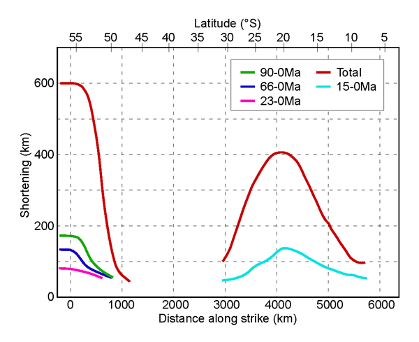
Figure 2. Variations and timing of along strike shortening in the Central and Southern Andes.
Data for the Southern Andes and Patagonian Orocline (between latitudes 58°S and 48°S) derived from Kraemer (2003). Data for the Central Andes and Bolivian Orocline (between latitudes 30°S and 10°S) is modified from Kley and Monaldi (1998), McQuarrie, (2002), and Arriagada et al. (2008). The total shortening for the Patagonian Orocline includes data from the Early Cretaceous to present (data for the periods Early Cretaceous–90 Ma, 90–66 Ma, 66–23 Ma and 23–present), while the total shortening for the Bolivian Orocline is from 45 Ma to Present (periods 45–15Ma and 15–0 Ma). Shortening data for the Patagonian Orocline, derived from balanced cross sections (Kraemer, 2003), illustrates the high along-strike total shortening gradient that evolved as a consequence of the hinged-point, with greatest shortening occurring at the southern extremity of the arc. The majority of shortening occurred during the mid-Cretaceous. The results from Arriagada et al. (2008) illustrate a large degree of shortening between 15 and 45 Ma. Note: the shortening curves are cumulative.