3D Modeling: case study
We have created 3D move models of the sand experiments representing the setting of the Strait of Messina using MoveTM computer software package (by Midland Valley Exploration, Ltd.) at three different extension levels i.e. at 0.5cm of extension, 2.0cm and 3.5cm. These models help in the comprehension of the basic kinematics of the area. The results of these models are comparable with true seismic section of the study area (Argnani et al., 2009).
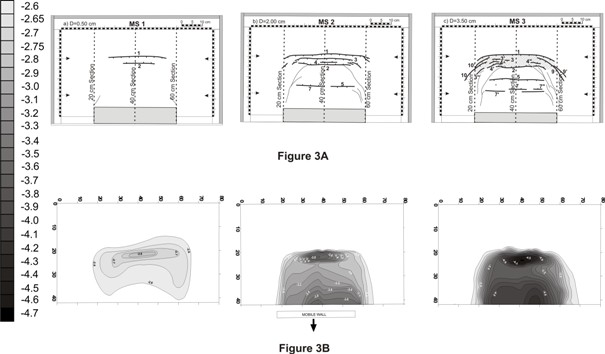
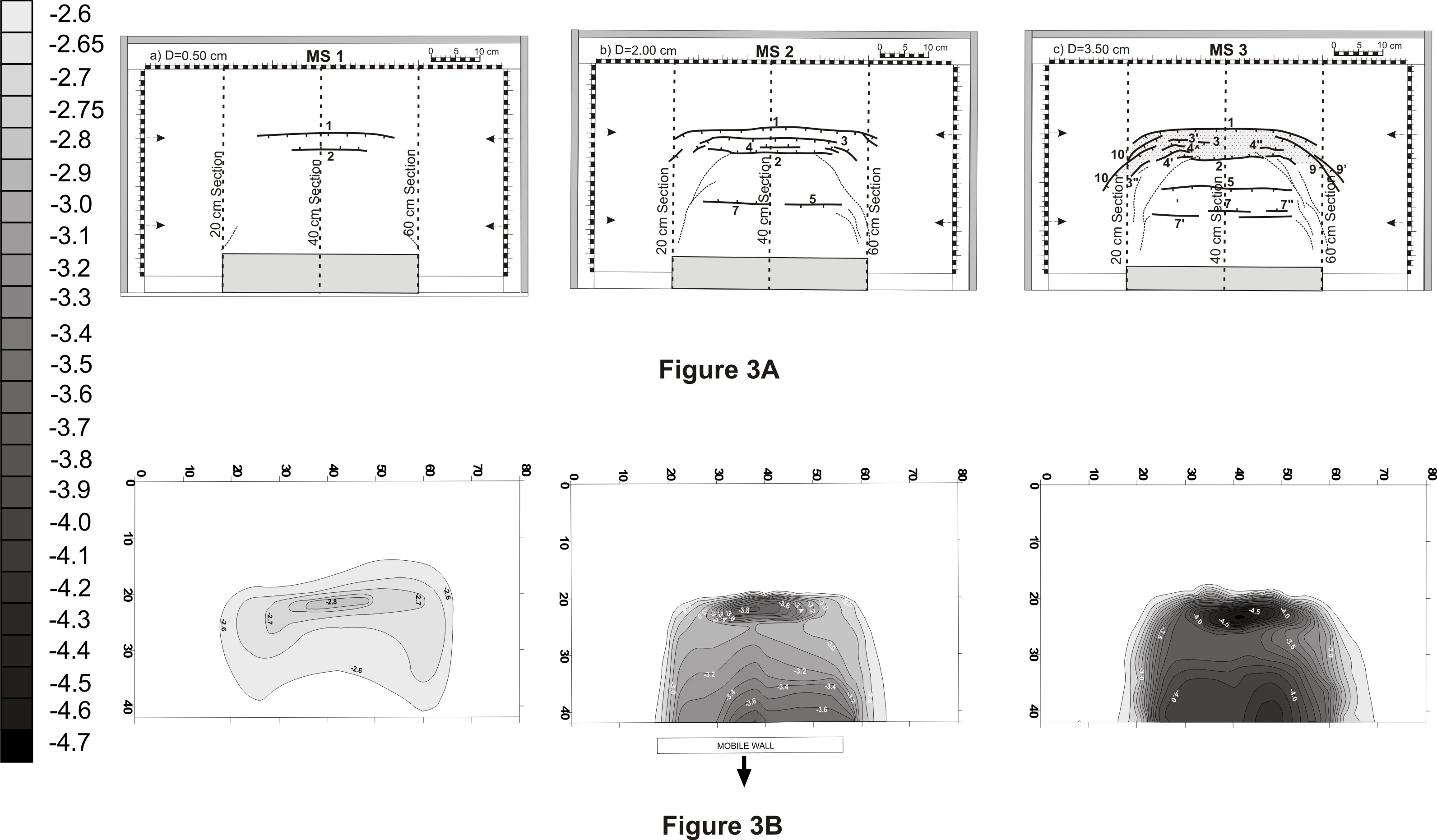
Figure 3 shows the generation of different faults with different extension levels. The first experiment was carried out on 0.5cm extension. A synthetic fault, visible in the central part, represents a surface expression of Messina fault, i.e. low-angle blind normal fault. After a few intervals an antithetic fault developed that is visible only in some central sections (from 36cm to 46cm) of the sandbox experiments. Both the faults have maximum displacement at 40cm cross-section area (i.e. in the middle of the sand-box). The progressive development of both faults and their lateral continuations are shown in Figure 3a.
In the second experiment, the total displacement is 2.0cm. In this experiment four faults are generated. They create a central graben and have the attitude shown by Figure 3b. The first (synthetic) and second (antithetic) faults are similar to those of the first experiment. The third fault is again a synthetic fault while the fourth one is antithetic. These all are high-angle normal faults produced as a result of displacement along the low-angle Messina Fault (<30°). When allowed to continue, a fifth fault is generated with a synthetic attitude in the right side of the experiment and resultant antithetic fault (fault 7) also in the same area. The last two faults are visible only in some parts of the experiment as shown in Figures 3a and 3b.
The third experiment underwent 3.50cm of extension along the fault plane and shows a major number of faults. Two grabens are developed in this experiment; one deep graben is on the central part while the second one is closer to the mobile backstop. The central graben is made up by dominantly two first-order faults (fault 1 and fault 2) and with some second order faults (fault 3 and fault 4). Presence of deep graben with high displacement along the fault planes indicates tectonic instability. The second graben is made by fault number 5 (synthetic fault) and 7 (antithetic fault). These faults are also visible in the experiment Ms2 but now they create a complete graben.
Figure 3. Generation of different faults and topographic surfaces
A) Development of different faults in different stages of experiment showing the position of internal sections at 20, 40 and 60cm (traces in the picture). Internal sections are 2cm spaced. B) Topographic surfaces with contour lines. The maximum depth of the central graben is -0.2cm in MS1, -1.2cm in MS2 and -2.2cm in MS3.
Animation A-2. Fault generation
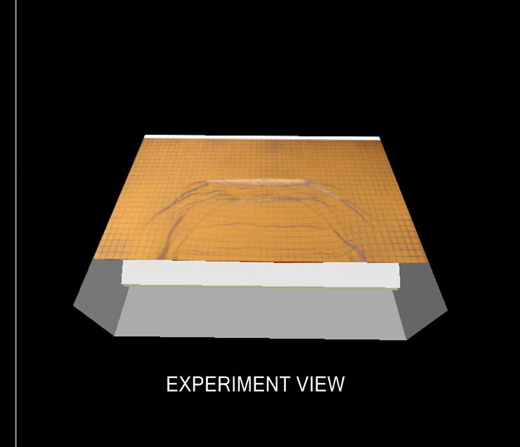
Generation of different faults in sequence and topography with experimental view and map view explaining the location of graben with respect to their actual positions.
Due to the similar patterns and the evolution of faults in the different models, we can say that these three models are like different steps in a single experiment with increasing amounts of displacement. The number of faults increased with the increasing extension along the fault plane. The generations of faults in different stages in the third model are explained in animation 2. This movie represents the formation of the grabens and shows changes in topographic surface accordingly.
These models have sections at 2cm intervals, perpendicular to the direction of the moving wall. In different stages of the experiment the sections show distinct faults. A 3D model built by interpolating these parallel sections can be used to to get more realistic fault shapes, for example the curved shape fault. Sections that are from 20cm to 60cm are more informative because of the size of the moving wall.
Animation A-3. The internal section of the experiment
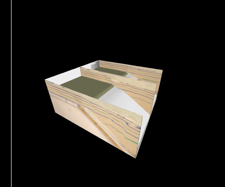
The displacement along the surface expression (fault 1) of the low angle normal fault is highest as shown in central section. Yellow lines are relative to topographic surface.
As has already been stated, 3D modeling allows one to visualize and manipulate geological model in real-time. Structural modeling has traditionally been carried out in 2D using cross-section interpretation as starting point. In 2D models there are some limitations; for example, in Figure 3 the real displacement along faults can be calculated along the 40cm section as it is normal to the faults, but in the same figure it cannot be calculated along 20cm and 60cm sections due to the curved shape of faults. For solving this problem we need a three dimensional tool that can also account for depth. Three-dimensional modeling offers both inclined shear and flexural slip information with strain visualization and displacement analysis.
There are many tools in 3D modeling for different types of analysis including Allan Mapper, an important tool for studying the displacement along the fault plane. It allows the footwall and hanging wall cut-offs to be mapped onto the fault surface as lines, as shown in Fig. 4. This software calculates all the values like the slip, heave and throw of a fault in an automatic way. Allan Mapper can be used to produce a separation map of the fault, which can then be used to restore faults with variable heave.
Figure 4. Cut-off lines on the fault plane
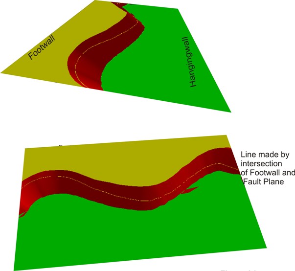
Figure showing the automatic construction of the cut-off lines on the fault plane (red surface). Starting from these lines, 3D Move software can automatically calculate the fault displacement.