The plate reconstructions proposed in this paper were made using an interactive software tool for plate tectonic modeling designed by the first author [PCME, Schettino, 1998]. This program also allows to plot relative or absolute velocity and acceleration fields for a given rotation model. If A and B are two conjugate plates and we indicate the instantaneous Euler vector (or angular velocity) of A relatively to B at time t as ΩAB = ΩAB(t), then the relative velocity field between these plates at an arbitrary location r is given by:

Hence, in order to calculate a velocity field, we need an estimate of the angular velocity for the considered time t. This estimate is accomplished as follows. A finite rotation pole is a representation of the orthogonal transformation matrix RAB(tk) that is necessary to move a plate A from its present location to a position with respect to plate B at time tk [e.g., Cox and Hart, 1986]. Typically, in the case of Mesozoic and Cenozoic models, times tk correspond to chrons associated to identified magnetic anomalies. Two successive times tk and tk+1 (tk > tk+1) are respectively the lower and upper age limits of a stage. If we consider the reference plate B as fixed to its present day location, the relative motion of A during a stage [tk,tk+1] can be described through a stage pole matrix SAB(tk,tk+1), given by:

This quantity represents the rotation that is necessary to carry a plate A from the position assumed at time tk to the position assumed at time tk+1 relatively to a reference plate B which is kept fixed in its present day location.
It must be pointed out that a stage pole matrix does not represent an instantaneous axis of rotation for the motion of A relatively to B between times tk and tk+1. In fact, by definition the plate A is considered at rest in the present geographic reference frame, whereas any instantaneous rotation of B with respect to A at time t ∈[tk,tk+1] must be calculated relatively to the "correct" location of A at that time. An interesting property of the stage poles is that by Equation (2) we can calculate an unknown finite rotation of A relative to B at time tk+1, provided that the finite rotation at time tk is known, and an estimation of the stage pole matrix between tk and tk+1 is available. In fact,

We will see that this Equation plays a key role in the description of the kinematics of the Mediterranean region. An estimation of the instantaneous angular velocity ΩAB at time t can be obtained as follows. We first calculate the stage pole vector eAB(tk,tk+1) and the stage angle associated to the matrix SAB(tk,tk+1). This pole represents the point of intersection between the rotation axis corresponding to SAB(tk,tk+1) and the Earth's surface, whereas the stage angle represents the total rotation angle about this axis. If we now rotate the vector eAB(tk,tk+1) using the total reconstruction matrix for the reference plate B at time t, the resulting vector represents the instantaneous Euler pole ωAB(t) at time t. Finally, in order to obtain the angular velocity rate ΩAB we divide the total stage angle by tk-tk+1.
The method described above allows to calculate velocity fields for any time in the geologic past, provided that a rotation model is available for the considered time period. It also allows to detect discrete variations of the velocity fields at stage boundaries. These variations are representative of acceleration fields and corresponding stress fields that act on the lithosphere at the transition times between two successive stages. The acceleration field between two plates A and B at the transition time t is defined as:

where δt represents a short time interval about the considered stage boundary (e.g. 0.1 Myrs). It should be noted that the term "transition time" refers here to any stage boundary in the rotation model that modifies one or more relative velocities along a circuit path. For instance, if plates A and B are related in the model through a third plate C, an acceleration between A and B may result either from a stage boundary between A and C or a transition between C and B.
We can now illustrate the theoretical framework that was adopted for the reconstruction of the tectonic history of the Mediterranean region proposed in this paper. In the following discussion we assume that the motion of intervening slivers at the interface between two main colliding plates is subject to precise physical laws that require periodic changes in the boundary geometry and formation of broad deformation zones. These changes have the primary role in restoring a state of equilibrium at the trench systems, in response to temporal variations of the main velocity field.
Consider an oceanic plate A that is subducting beneath a plate B. At the equilibrium the net torque exerted on the plate boundary is zero, because all the forces applied at the trench zone are balanced (Fig. 4a). In this instance, the subduction rate is determined by the relative velocity of A with respect to B. Suppose now that a sudden change of the absolute velocity of A (the velocity of A with respect to the deep mantle) occurs that determines a decrease of its velocity relatively to B (Fig. 4b). An analogue situation could be represented by two persons that are pushing one another, and by a subsequent sudden release from one of the two opponents. The resulting predictable conclusion would be an unbalancing of the other one and thrusting toward the retreating person. In the case of two plates the unbalancing would generate a tensional stress field at the margin of B which may activate a subsequent process of back-arc deformation.
Figure 4. Sketch illustrating two different scenarios for the formation of slivers
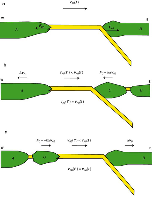
A: Starting configuration. The trench system is in a state of equilibrium at time t. B: At time t' plate A accelerates away from the trench. The resulting tensional stress field at the trench causes back-arc spreading in marginal areas of B. C: In a different scenario an eastward acceleration of plate B determines rifting at the continental margin of the conjugate plate and the formation of the proxy sliver C.
A somewhat different situation would occur if the retreating block coincides with the upper-plate. In this instance, a tensional stress field would be applied to the subducting plate (Fig. 4c) and transferred to the deformable continental margin of A. Therefore, the oceanic part of this plate would be decoupled from the undeformed continent and a small fragment of continental lithosphere would travel toward the trench along with the surrounding oceanic crust. In both scenarios, a force F = kΔv is applied to the continental fragment with a magnitude proportional to the variation of relative velocity.
This model may explain several kinematic features of the subduction process in the Mediterranean region, in particular the rifting of continental terranes from the northern margin of Gondwana during the Mesozoic and the formation of extensional basins during the Cenozoic (Balearics, Tyrrhenian, Aegean, etc.). For instance, when Africa accelerated eastwards at chron 7 (25.2 Ma) about a pole located at (78.81N,301.25E), this retreat from the former Iberian trench may have resulted in the rifting of Sardinia, Corsica, Calabria and the Balearics from the Iberian margin between chrons 7 and 6. However, in this paper attention is focused on the kinematics of the Mediterranean region during the Mesozoic, which was dominated by the fragmentation of the northern Gondwana margin by successive retreat of the overriding plate (Fig. 4c) and by intermediate stages of trench compression.
A simple method for calculating finite rotations of continental fragments that traveled from a passive margin towards a trench is based upon the concept of decoupling of the oceanic part of a plate by fragmentation of the adjoining continental margin. As illustrated in Figure 4c, the new oceanic plate retains the subduction rate as an invariant of the process, and the whole mechanism allows the trench system to restore the state of equilibrium when the transition to the new stage is completed. Hence, the stage pole of the new plate with respect to the upper plate for the successive time period must coincide with the former stage pole of the subducting and still undeformed lower plate. Moreover, conservation of the subduction rate is required for any subsequent stage. This observation implies in general that successive small variations of the relative velocity between A and B will be compensated by different spreading rates at the ridge that separates the additional plate C from A. However, a strong acceleration of A in the direction of B could not be compensated by a lower spreading rate. In this instance, the ridge would collapse determining the formation of ophiolites [Robertson and Dixon, 1984].
In order to calculate finite rotations for the Mediterranean microplates, Equations (2) and (3) will be applied iteratively, starting from the initial stage associated to the early formation of oceanic crust in the Central Atlantic and from the assumed initial assemblage at the Northern Gondwana margin. It will be shown that the stage pole associated to the subduction of oceanic lithosphere beneath the Eurasian margin between 175.0 Ma and 170.0 Ma was conserved until chron M0 (120.4 Ma), when an abrupt change in the relative motion of Africa with respect to Eurasia determined the onset of the Alpine collision. During this long time period a unique stable system comprising a stationary trench in the Northern Tethys and a buffering spreading center to the South existed. According to the theoretical model discussed above, this process can be viewed as the driving mechanism for the drifting of Northern Turkey towards the Eurasian margin.
In the following sections the fourteen stages that characterized the tectonic history of the Mediterranean region during the Jurassic and the Cretaceous will be grouped in nine major phases. For each phase boundary, reconstruction maps will be discussed that show the velocity and acceleration fields, the modeled pattern of seafloor spreading [Schettino, 1999] and the distribution of the continental lithosphere. The geomagnetic time scales of Cande and Kent [1995] and Gradstein et al. [1994] are used respectively for anomalies younger than chron 34 (83.5 Ma) and for older times. A full animation of the paleogeographic evolution of the Tethyan realm is shown in the Appendix and is also accessible through the Internet at: http://www.serg.unicam.it/Geo.html [Schettino and Scotese, 2001].