Data Analysis

Experimental Data

Raw Data
To examine the strain distribution in the model, the deformation field has to be analysed. The movement of passive markers can provide the necessary information. These markers can either be small particles or a passive grid inscribed into the wax. The markers need to act passively during the deformation of the model, i. e. they must neither give additional strength nor show movement of their own (e. g. gravitationally). Furthermore, the markers should provide a good optical contrast with the surrounding material to be visible and identifiable on photographs.

In the experiments presented here, a passive grid was used to visualize the bulk deformation during the experimental phase. Because of melting in the lowermost part of the experiment, parts of this grid lost contrast during deformation. Therefore, small (??1 mm) coloured plastic particles were added to increase the number of markers. Nevertheless, markers that left the visible domain (in wax melting at the model base or moving behind the pistons) could not be used. The total number of markers (particles and grid points) in each experiment was between 160 and 640.

Optical images were taken during the deformation using a black and white digital camera. These images show the side view of the analogue models. After each experiment, it was verified that the deformation was homogeneous in the line of view, i. e. that the images represented the deformation within the model.

Simultaneously with the optical images, infra-red images were recorded. They offer a theoretical resolution of 0.3 K, but due to the necessary calibration described by Wosnitza et al. (2001) the error is about 2 K.

Data Preparation
Before data analysis, the optical images had to be processed. All the markers visible on each of the successive photos were selected and were assigned a number, using an image processing software (Adobe Photoshop). Subsequently, the positions of the markers were digitized on the computer screen using routines of plot_grid (Mancktelow, 1991). The markers of each block of material were digitized separately to allow for movement along the block interfaces.

From the coordinates of the markers within each block of material, a Delaunay Triangulation (the smallest occurring angle is as large as possible, Wolfram 1991) was calculated, and triangles with lines outside the block were removed using a routine from Sedgewick (1988). The triangulation of the initial stage of the experiment provided the connectivity list for all other subsequent time steps. This topology was followed through time, and the change of its geometry was analysed.

In this analysis, the overall strain can be considered as being homogeneous within one triangle. All subsequent considerations refer to the deformation of the single triangles.

The experiments show no significant inhomogeneities in the third dimension, perpendicular to the transport direction. Therefore, the deformation in this direction can be neglected, and a two-dimensional approach is sufficient.

Strain Analysis

In an area of homogeneous strain, the deformation can be described as linear coordinate transformation. In general, this transformation can be split into translation, rotation and deformation.

Strain Matrix
Disregarding translation, the Lagrangian formulation of the coordinate transformation equations in two dimensions is

(2.17)

which leads to the strain matrix ε defined by

(2.18)

(Ramsay & Huber, 1983), where

(2.19)

The relative movement of the three vertices of a triangle can be used to determine the strain matrix for that triangle. For this, the coordinates of two vertices are expressed relative to the third, which is taken as the origin. Thus, movement of the whole triangle does not contribute to the internal deformation. For a triangle defined by r₀, r₀ + r₁ and r₀ + r₂ (see Figure 4) the deformation matrix ε can be found solving

(2.20)

simultaneously. This is possible as long as r_i are not parallel, i. e. the triangles enclose non-zero area.

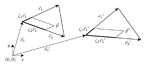Figure 4. Triangle before and after deformation From the transformations r1→ r1' and r2→ r2', various strain properties can be calculated. The coordinates of a point p within a triangle can be expressed in terms of the sides of that triangle. Those pseudo-coordinates ζ1 and ζ2 do not change, as long as deformation is homogeneous in the domain in question. (Click for enlargement)

Strain Ellipse
The angle between the coordinate axes and the principal strains can be found from the entries of the strain matrix using

(2.21)

(Ramsay & Huber, 1983).

A useful way to visualize strain is the strain ellipse (Ding, 1984). It shows the deformation of a circle inscribed on the object in question. Knowing the strain matrix ε, the properties of the strain ellipse can be calculated. The equation defining the strain ellipse is

(2.22)

(Ramsay & Huber, 1983). By rotating (x',y') in equation 3.6 back to (x, y) using a rotation matrix around ϑ from equation 3.5, the principal strain axes and the coordinate axes coincide. The principal strains e_x and e_y can now be obtained from the coefficients (1 + e_x) and (1 + e_y) of x² and y² respectively. For visualisation, the ellipse is plotted by using the parametric variable χ ∈ [0°,360°]:

(2.23)

The angle χ is a parametric variable which does not refer to a physical surface. It should not be confused with the angles in stress ellipses or Mohr circles.

Other Strain Properties

Rotation
The angle by which a material line, that coincides with one of the principal strain axes, is rotated is given as

(2.24)

(Ramsay & Huber, 1983). This angle is a measure for the amount of simple shear in the deformation. In the case of pure shear, ω = 0°, while for simple shear 0 < |ω| << 90°, where the positive sign represents sinistral sense of shear. The definition of rotation is similar to that of the "vorticity number" W_k by Means et al. (1980), leading to comparable characteristics for the two properties.

Ellipticity
The ellipticity of the strain ellipse can be found by dividing the two principal stretches:

(2.25)

Dilatation
The dilatation is the determinant of the strain matrix minus one, or

(2.26)

(Ramsay & Huber, 1983). That is, the dilatation is the relative change of area. A dilatation of zero therefore corresponds to no change of area, dilatation of one means doubling of the area. Negative dilatations between minus one and zero correspond to a reduction of the area. Dilatations smaller than minus one indicate flipping of the triangle in question along one of its sides.

Strain Tensor
The strain matrix ε also relates to the displacement gradient matrix ∂u_i/∂x_j as

(2.27)

and the strain tensor ε_ij is the symmetric part of the displacement gradient matrix

(2.28)

(Ranalli, 1987).

The strain tensor can be split into its isotropic and deviatoric parts ε_ij = ε_isoij + ε_devij (Etchecopar et al., 1981). The isotropic strain represents the volumetric dilatation and can be expressed as the mean of the diagonal elements:

(2.29)

Note that in the case of small deformations (a - 1, d - 1, b, c << 1), ε _iso = Δ.

Stress Analysis

Viscosity
As mentioned above, the temperature distribution in the model could be recovered from the infra-red data. For the materials used in these experiments the function η(T) was known. Using the Arrhenius Equation 2.15 and the data given in Table 7 allow to calculate the viscosity η from the temperature T.

The basis for these temperature data were the infra-red images, each consisting of 300 x 200 pixels. The "window" of the experiment contained about 290 x 130 pixels. In practice, the calculation of the viscosity was made for each pixel. The viscosity was then averaged for the triangle used to determine the deformation (on average about 60 pixels per triangle). Together with the strain tensor, the viscosity allowed to calculate the stress within the model.

Stress
For Newtonian materials, the relationship between the strain rate tensor and the stress tensor is given by

(2.30)

where the viscosity is scalar. Thus, the two tensors have the same mathematical properties, only the eigenvalues differ in the factor η.

The stress tensor links a surface normal n to the traction r_n acting on that surface via

(2.31)

(Ranalli, 1987).

A vector which, when transformed with a tensor, remains its direction and only changes its length is called an eigenvector to that tensor. The change of length is called the eigenvalue (Kowalsky, 1979, r≠0).

The eigenvectors of the strain tensor coincide with the principal axes of the strain ellipse and represent the principal strains (Ramsay & Huber, 1983). The eigenvectors of the stress tensor represent the principal stress directions, the eigenvalues σ_i represent the absolute values of the principal stresses where σ₁≥σ₂≥σ₃ by convention (Ranalli, 1987). The principal strain axes and the principal stress axes coincide in pure strain, a simple shear component leads to angles in the range ±45° between principal strain and stress axes.

Similar to the strain tensor, the stress tensor can be split into its isotropic and deviatoric parts. If the material is considered to be incompressible, only the deviatoric stress contributes to the strain, and the isotropic strain is zero. In the experiments presented here, melt could move within the model (cf. Barraud et al., 2000). Consequently, some triangles could gain or lose volume and the isotropic strain was non-zero so that absolute stresses could not be calculated. Nevertheless, addition of an isotropic component to a tensor does not alter its eigenvectors. The eigenvalues do change, but the difference between any two eigenvalues remains the same.

For visualisation, the differential stress (σ₁ - σ₃)/2 and the direction of σ1 are given in the Appendix. Note that the term "differential stress" should not be confused with "deviatoric stress" (Engelder, 1994). The former denotes the scalar difference between maximum and minimum principal stress, whereas the latter is a tensor with the sum of its main diagonal elements being zero. Deviatoric stress and differential stress can only be equal under isotropic stress conditions.

PT t Paths
Under certain conditions, the pressure-temperature-time history ("PTt path") of a rock sample could be deduced (e. g. Thompson & England, 1984). It was also possible to obtain the PTt path for given material points in the analogue experiments presented here. Because of the problems concerning scaling of temperature as described in section 2.4, the temperature paths for the model material points are more qualitative than quantitative. Nevertheless, a rough temperature scale can be given, as described in section 2.2.3.

To be able to choose arbitrary material points, movement has to be interpolated from the known deformation field. Firstly, the triangle containing the initial point p has to be found. The coordinates of p can be expressed in terms of the corners r₀, r₀ + r₁ and r₀ + r₂ of that triangle (see Figure 4) by solving

(2.32)

for ζ₁ and ζ₂. This is possible if the triangle has non-zero area.

Since the deformation is assumed to be homogeneous within the triangle, the "coordinates" (ζ₁, ζ₂) of p are constant during deformation.

The temperature of the material point can easily be inferred from the position and the temperature distribution. For the pressure, only the lithostatic pressure was given. Omission of "tectonic" differential stresses is also usual in petrological studies, where pressure from PTt paths is converted to depth (e. g. Jamieson & Beaumont, 1988). Nevertheless, tectonic stresses might exceed the lithostatic pressure under certain conditions (Mancktelow, 1995).

The load of material above p is calculated by finding the material boundaries above it, and multiplication of the resulting heights with the respective densities following

(2.33)

Implementation

The implementation of the analysis described above was achieved quite straightforwardly using the software "Mathematica" (Wolfram, 1991). Preliminary steps include digitisation of the marker positions at several time frames, triangulation and removal of triangles "outside" of the experimental domain.

Strain could be calculated incrementally during a time step, or as finite deformation relative to the initial state. The former was needed for later analysis of the stresses, the latter was advantageous for visualisation of the progressing deformation. Thus, starting from the coordinates of a triangle at two points in time, the following procedure was carried out:

1. Equation 3.4 solved for ε.

2. (x', y') rotated back to (x, y) by angle ϑ (equation 3.5) in the ellipse equation 3.6.

3. From the resulting equation, the coefficients of x₂ and y₂ were extracted to find theprincipal strains.

4. Strain ellipses plotted using equation 3.7.

5. Dilatation plotted using equation 3.10.

6. Rotation plotted using equation 3.8.

7. Ellipticity plotted using equation 3.9.

8. Viscosity averaged over each triangle.

9. ε_ij calculated from ε using equation 3.12.

10. σ_ij calculated from ε_ij using equation 3.14.

11. Eigenvectors of σ_ij calculated.

12. Differential stress calculated from σ_ijj.

13. Differential stress plotted.

14. Direction of the principal stresses (eigenvectors of σ_ij ) plotted.

All these steps should be taken literally. With "Mathematica", modification of an equation by a coordinate transformation is as easily done as extraction of coefficients from the resulting equation or the calculation of eigenvectors of a tensor.