Parameters Scaled

Time, Velocity and Length
In these experiments advantage was taken of the differences in rheology induced by the thermal gradient within the material. One of the main demands on scaling was therefore that thermal velocities were scaled by the same factor as mechanical velocities.

The equation governing heat transfer in thermally isotropic materials, without internal heat production, is

(2.1)

During deformation, thermal and mechanical velocities must be treated equally. Thus, it must be ensured that the time needed by material particles or heat to move over a certain distance is scaled by the same factor. For the scaling factors of length l, time t and thermal diffusivity κ,

(2.2)

can be obtained, where the scaling factors S_X of a property X represent the ratio of laboratory values to natural values. Equation 2.2 couples the length and time scales to the material-dependent scale of thermal diffusivity.

The length and time scales are also coupled by the request for kinematic similarity. All velocities in the model must be scaled by the same factor

(2.3)

The thermal diffusivity of rocks is about 10^-6m²s^-1 (e.g. Ranalli, 1987; Fowler, 1990, ch. 7), whereas that of paraffin wax is about 8x10^-8m²s^-1 (Rossetti et al., 1999). This results in a scaling factor Sκ of 8x10^-2. Orogenic convergence rates are in the range 1-5cm/a (e.g. Pfiffner & Ramsay, 1982). The experimental convergence velocities 8-10µm/s chosen for the experiments are therefore scaled by 2.5x10⁴. From the resulting scaling factor for time of 1.26x10^-10, and using equation 2.3, the scaling factor for length is found to be 3.17x10^-6. As a consequence, the initial model length of 45cm corresponds to a length in nature of about 140km, and one hour of experiment time corresponds to a geological time of 0.9Ma.

The scaling of length is limited by the size of the smallest particles used in the experiments. The grains of the brittle material used are smaller than 200µm, which scale to 63m in nature. The process of the data analysis (Part 3) uses markers with a spacing of the order of centimetres, limiting the interpretation of the experiments to lengths larger than 3 km.

Viscosity and Stress
In the model, as in nature, gravity g acts on a material unit with a density ρ and a thickness h, resulting in gravitational stresses σ_grav. Gravitational stresses need to have the same scaling factor as viscous stresses σ_visc, where the latter result from deforming a material with a linear viscosity η at a strain rate ε. Because of

(2.4)

and

(2.5)

the model is only scaled to gravity when

(2.6)

This also implies the scaling factor for stresses to be

(2.7)

In experiments, where the length and time scales are only coupled by limitations for the scaling of velocity, equation 2.6 can be used to vary the scaling factor for time. In these cases, a centrifuge is needed to vary S_g (e. g. Koyi & Skelton, 2001; Koyi, 2001).

The mean densities of the upper and lower crust are 2800 kg/m³ and 3300 kg/m³, respectively (Fowler, 1990). The densities of the according analogue materials Jet-Plast and paraffin wax are 736 kg/m³ and 882 kg/m³. The resulting scaling factor for density Sρ = 0.26 applies for both upper and lower crust. Using equation 2.6 and 2.7, scaling factors for viscosity and stress are found to be Sη=10^-16 and Sσ=8x10^-7.

The scaling factor for viscosity can be used to determine the viscosities needed in the analogue model. For this, the viscosities of natural rocks must be calculated from published flow parameters and an assumed geothermal gradient. Using a geotherm of 20°C/km typical for a convergent collisional orogenic setting (e. g. Decker et al., 1988), a wide range of viscosities can be found. Basing on parameters from Carter & Tsenn (1987) for "wet" dunite and a temperature of 720°C at a depth of 35km, a viscosity of 3.1x10²² Pa s is obtained for the top of the upper mantle. Scaling this value to the laboratory using Sη = 10^-16, the viscosity for the wax needs to be 3.5MPa s. This viscosity can be reached using the paraffin wax P57 at a temperature of 42.3°C, which is close to the melting point of the other paraffin wax (P43). In order to have the base of the upper mantle as weak as the base of the lower crust, a temperature of around 56°C must be set at the model base. Since the above depth of the Moho scales to 11 cm in the model and an overall lithospheric thickness of 60km scales to a model height of 19 cm, the required thermal gradient in the experiments turns out to be 1.7°C/cm. These arguments leads to the viscosity profile for the model shown in Figure 3.

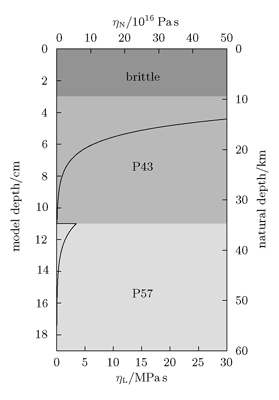Figure 3. Rheological stratication in the experiment. In the top layer, the Jet-Plast shows Mohr-Coulomb rheology. The viscosities of the two wax layers are determined using the parameters presented in Table 7. The viscosity contrast at the depth of 11 cm is about 4MPa. Note that the horizontal scale gives viscosities instead of fracture strengths. The latter are commonly found in the literature (e. g. Ord & Hobbs, 1989; Handy et al., 2001; Kirby & Kronenberg, 1987; Carter & Tsenn, 1987), but are inappropriate for viscous (Newtonian) materials. (Click for enlargement)

According to Weijermars & Schmeling (1986), rheological similarity also demands equality of the dimensionless stress exponents for natural and analogue materials. This exponent is between 1.8 and 5.1 for the materials shown in Table 2. For the paraffin waxes used, the measured data is consistent with n = 1. Rossetti et al. (1999) obtained similar low (n < 1.3) stress exponents, while Mancktelow (1988) gave values between 2.4 and 4.1. This value is only significant in scenarios with large gradients in the strain rate.

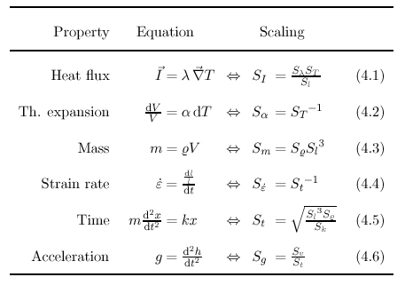Table 1. Additional equations for scaling of thermomechanical analogue experiments. These equations are not considered in the experiments presented here. The effects involved are negligible (4.6, 4.5), do not contribute to the deformation (4.1), or they are trivial (4.3, 4.4).

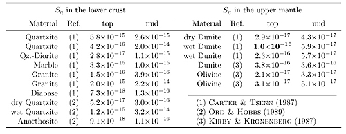Table 2. Scaling of viscosity. Depending on the parameters for the materials chosen, different rheological scenarios are possible. In this table, the scaling factor for viscosity Sη is given for various earth materials in different depths (top and middle of lower crust and upper mantle). The values were calculated from properties given in the references. The scaling factor of 1.0x10-16 as calculated from the scaling factors for length, time and density is reached for wet dunite at the depth of the top of the upper mantle. Furthermore, the model turns out to be scaled for a lower crust composed of granites, which is plausible.

Temperature
To check the scaling factor for the absolute temperature T, consider the temperature-dependent flow law for polycrystalline aggregates. This relation is often expressed in power-law form as

(2.8)

or more commonly as

(2.9)

where

(2.10)

(Means, 1990). This equation does not influence the scaling factors for stress or strain rate, but it requires the exponent

(2.11)

to be dimensionless. Because of S_R = 1,

(2.12)

The activation energy for the paraffin waxes used was measured to be about 420 kJ/mol (see Table 7). For the dunite mentioned above, around 500 kJ/mol were given by Carter & Tsenn (1987). This results in a scaling factor for the activation energy of 0.84. The ratio of the absolute temperatures at the "Moho" (315 K in the model, 1000 K in nature) is 0.3. Therefore, temperature is not correctly scaled. Since the activation energy influences the curvature of the profile shown in Figure 3, correct scaling of the temperature should cause the profile to bend more sharply. Consequently, the scaling of the viscosity is correct at the depth of the Moho only. Table 2 gives the actual scaling factors for viscosity for different depths and different parameters, resulting in values for S_η between 7x10^-18 and 3x10^-14. The variation at a constant depth of up to three orders of magnitude is due to variations in the measured parameters for lithospheric rocks. Furthermore, the data for natural rocks is gained from samples which are small compared to the areas modelled, which contributes to the uncertainties (Handy et al., 2001).

Using materials with lower activation energies such as colophony (Cobbold & Jackson, 1992, H = 255 kJ/mol) would improve the quality of scaling. Materials with a larger activation energy such as the paraffin used by Rossetti et al. (1999) result in a required scaling factor for temperature larger than one. In that case, the temperatures in the laboratory should be larger than those in nature, in order to provide correct scaling.

However, following an argument of Cobbold & Jackson (1992, p. 257), only the first two or three orders of magnitude of the overall strength variation are likely to have significant mechanical consequences. Whether the weaker layers are weaker by four or by five or even more orders of magnitude does not influence the stiffness of the overall scenario. Therefore, an attempt to perfectly scale the experiments for temperature is probably unnecessarily rigorous.

Nevertheless, "pseudo-temperatures" may be given for the model. These temperatures can be used in PTt paths (see sections 3.3.3 and 4.2.5). To scale a model temperature T_L to nature, the following "work-around" for the scaling of temperature is proposed:

(2.13)

Here, the thermal gradient in the laboratory T_L(z_L) is used to calculate a corresponding "depth" z_L . Using the scaling factor for length S_L, z_L is converted to a natural "depth" z_N. From the latter, the natural temperature can be reconstructed using T_N(z_N). "Depth" in this context is not to be taken literally since it describes the depth in a scenario with a homogeneous geothermal gradient. Instead of a simple scaling factor, the proposed work-around provides the linear relationship

(2.14)

This approach has certain drawbacks:

• Phase transitions in either material are ignored, although they are essential in the reconstruction of natural PTt paths. Phase transitions also influence the overall rheology of crustal and mantle materials.
• In some cases, unrealistically low temperatures are obtained for the upper crust. This is due to the thermal conductivity of the brittle material which is different from the conductivity of the waxes.
• The incorrect scaling of temperature does not only obstruct the direct way from T_N to T_L. It also causes the flow laws in the laboratory and in nature to be not exactly similar. Thus, only in the stronger parts of the materials does that relationship hold.

Therefore, the temperatures obtained this way should be used with caution. Nevertheless, at the present stage of this work, this is the only way to gain temperature predictions from the analogue experiments.

Brittle Behaviour
The rheological behaviour of brittle rocks can be described by using the angle of internal friction and the cohesion σ_c to determine the fracture strength σ_f from the lithostatic pressure σ_lith

(2.15)

neglecting pore pressure effects (Hubbert & Rubey, 1959).

The angle of internal friction is dimensionless, therefore it must be equal in the model and in nature. Jet-Plast, the brittle material chosen has an angle of internal friction of (37±2)°. Natural brittle rocks show angles of internal friction of 25° - 35° (e. g. Lallemand et al., 1994). Although the scaling in this case is not perfect, the error bars overlap.

Cohesion is a stress, consequently it needs to be scaled with the scaling factor for stresses. According to Hoshino et al. (1972), crustal rocks show cohesions of <20 MPa. In fact, these values were measured for rather small samples (some centimetres height). Due to pre-existing fractures, the bulk cohesion of the upper crust might be lower. Sand has cohesions of 20 -170 Pa (Lallemand et al., 1994). Due to the composition of the Jet-Plast, electrostatic forces can be assumed to lead to a lower cohesion. The upper limit of the natural cohesions scales down to 17 Pa which is well in the plausible range for the model material.