 (a)
(a) 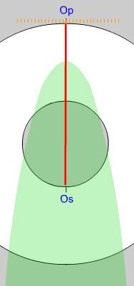 (b)
(b)
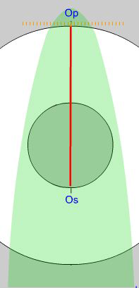
Figure 5. Parabolic failure envelopes for (a) total and (b) effective stress.
To illustrate the general Mohr-Coulomb type failure criteria on the new constructions, an area is shaded green as in Fig. 5; however, the shaded outline is now parabolic, representing the transition from brittle to ductile deformation mechanisms with depth in the earth's crust, and it extends past the trace of the plane, representing material with a certain tensile strength due to its cohesiveness (Fig. 5a).
Whereas the influence of pore fluid pressure is usually represented by drawing different Mohr circles for stress and effective stress, it makes more sense, following Bayly (1991) to shift the Mohr envelope instead. This is implemented in the animation linked to Fig. 5. When pore pressure is applied, the shaded area shifts away from the plane's trace, reducing the extend of the stable region. As the mouse is dragged around the doughnut, there are some directions in which the stress vector falls outside the shaded stable envelope. Pore fluid pressure is applied in the animation linked to Fig. 5 by clicking the lower right button.
The Construction for Two Stresses of Opposite Sign
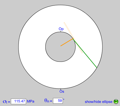
Figure 6.
Construction for stresses of unlike sign. Click
here to view animation.
The green shaded sectors of the stress ellipse represent the field of
tension this case.
When the principal stresses differ in sign (one being compressive, the other tensile), their sum is numerically less than their difference. In this case, therefore, the origin of planes, Op, lies on the inner boundary of the doughnut and the origin of stresses, Os, lies on the outside (Fig. 6). If you apply the same rules of construction as before, counting degrees clockwise from Op and counterclockwise from Os, or vice versa, the construction yields valid results. Now there are two special conjugate orientations in which the normal component of stress drops to zero; in these orientations, the stress vector is parallel to the trace of the plane and is equal to the shear stress component. These cases correspond to the points where the Mohr circle intersects the shear stress axis of a conventional Mohr Diagram and they divide the stress ellipse into fields of compression and tension, as color-coded in the animation.
The constructions presented thus far are ideal for determining the stress state given fixed values of the principal stresses. However, there are many situations in which it is desirable to examine variations in the stress tensor with time and for these, the classical Mohr construction is still superior; therefore, it is important to be able to transfer from one construction to the other.
The relationship between the doughnut construction and the Mohr Diagram could not be simpler to illustrate, since the inner circle of the doughnut is a rotated version of the Mohr circle; all you need do is lift the tracing overlay off the grid and reorient it with the plane's normal and trace oriented as abscissa and ordinate. Click here for an animation of this transformation or refer back to Fig. 4. Note the relationship between the Mohr circle's poles and the two origins of the doughnut diagram, Op and Os.
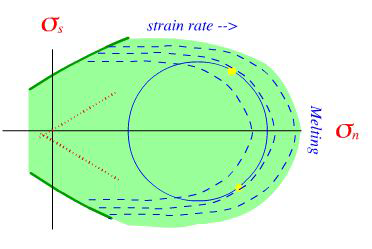
Figure 7. Animation of Mohr Envelope Constructions for (a) brittle deformation, (b) yielding failure, and (c) ductile shear.
The role of the traditional Mohr Diagram can be enhanced with the aid of animation, as illustrated in the Flash movies linked to Fig. 7. This is particularly true of sub-critical stress states early in a deformation history, which are difficult to illustrate with overlapping series of circles, and at elevated confining pressures, where rapid ductile strain rates lead to a dissipation of the applied stress difference. In Fig. 7a, a specimen (blue) is subjected to increased confining pressure in stage (1), represented on the Mohr diagram by a point (circle of zero radius) that moves across the normal stress axis. In stage (2), an axial load is applied via the red and black pistons, creating a differential stress represented by the radius of the growing Mohr circle. In stage (3), the specimen fails along a fracture plane (dash yellow line) determined by the point of tangency of the Mohr circle and envelope. The magnitudes of the nomal and shear stresses at the moment of failure are indicated by the red dot in stress space. Whether the plane show here or its conjugate (reflected through the vertical) becomes the site of specimen failure is a matter of chance.
Figure 7b shows an similar experiment in which the specimen yields just before failing, whereas in Fig. 7c, the period of ductile flow after yielding is prtracted. The differential stress that the specimen can maintain (which equals the diameter of the Mohr circle) is a function of strain rate, since strain dissipates the applied load by continuous flow on ductile shear zones (dashed yellow lines). The orientations of the ductile shear zones on which the specimen deforms and the stresses on the those shear planes (yellow spots) are determined by "Bayly Curves" (1991 - dashed) that contour strain rate, as indicated by the "strain rate -->" label. These curves are a function of the material and may be straighter, or even concave.