The Hand-drawn Construction for Uniaxial Stress
To create an equivalent construction using pencil and tracing paper, print Fig. 1 onto plain paper or acquire a polar grid and ruler, and then follow these steps:
(i) Mark a point Op on the perimeter of the grid at zero degrees which we will call the "Origin of Planes."
(ii) Mark a second point Os, also on the grid, at 180 degrees, which we will call the "Origin of Stresses."
(iii) Place a tracing overlay on the grid and draw an arbitrary radius to represent the normal to a plane of interest and a hashed tangent to represent the trace of the plane. The lengths of these radial and tangential lines have no numerical significance; they just mark directions. At the outset, the tracing overlay should be oriented so that these two lines intersect at the origin of planes, Op.
(iv) Let the diameter of the net represent the principal stress σ1 = 200 MPa. So, for example, if the net's diameter is 20 cm as in Fig. 1, then every bold (centimeter) division corresponds to 10 MPa and every smaller (2mm) division represents 2 MPa.
(v) To determine the total stress σt on a plane whose normal subtends an angle θn clockwise from vertical, rotate the tracing overlay clockwise through the angle θn from the origin of planes, Op, then count an angle -θn counterclockwise from the origin of stresses, Os (this mark is on the grid, not the overlay, so it does not rotate), and joint the resultant points.
Step (v) is a rather roundabout way of drawing a vertical line! However, it introduces the general procedure that must be followed in the more complicated cases that follow.
The line thus drawn represents the stress vector σt in magnitude and orientation. It's shear and normal stress components, σs and σn , may be found by casting perpendiculars onto the trace of the plane and its normal, and measuring the components with a ruler scaled to 1 MPa per millimeter in this case. Obviously, these stress components are also shown in their correct spatial orientation.
Generalization to cases of non-vertical principal stress is trivial; you simply rotate the two origins, Op and Os, and the tracing overlay, to the desired inclination. Using the Flash animation, you enter a value for θ0 and click the set button. Unlike the classical Mohr construction, there is no complicated procedure for relating data in geographic space to data in stress space.
Slip
on Preexisting Failure Plane
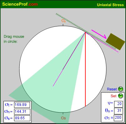
Figure 3. Flash animation of the failure criterion for slip on a preexisting plane. Click to interact.
The uniaxial stress construction is immediately ready for practical application. Let the angle of sliding friction for slip on a preexisting fracture or fault plane be ψ = 20 degrees (correspondingly, the coefficient of sliding friction is μ = tanψ ). We can shade an area analogous to a pre-fractured Mohr-Coulomb envelope, shown in green in Fig. 3. In the hand-construction, this shading is applied on the overlay so that it rotates with the plane's trace and normal. Using the flash animation that is linked to Fig. 3, enter the desired angle of friction in the ψ text field and press the set button. Then either drag the mouse to change the plane's orientation or enter its dip in the θn text field and click the set button. As long as the red stress vector lies in the green stable field, a block resting on the plane is stable. As soon as the dip angle exceeds the angle of friction, the block slips. [Astute students may question why the block does not accelerate. This is mainly due to author's laziness but also reflects the block's terminal velocity under frictional sliding. The block does slide faster at steeper dips but does not fall off after 90 degrees; no useful purpose, beyond entertainment, would be served by such an animation enhancement.]
By reducing the value
of the principal stress in the σ1 text field, you can
powerfully convey the fact that, in this cohesionless scenario, sliding
can occur no matter how small the shear stress magnitude, provided the
shear to normal stress ratio exceeds the coefficient of friction, μ.
The Construction for Two Stresses of Like Sign
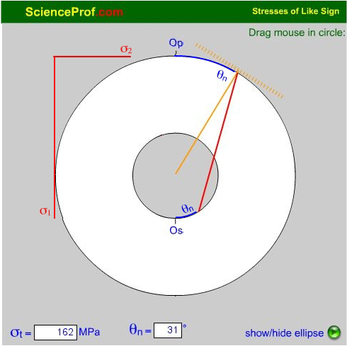
Figure 4. Construction for stresses of like sign.
See text for explanation. Click
here for animation.
A more general case is represented in Fig. 4, where two principal stresses, σ1(vertical) and σ2 (horizontal), are either both compressive or both tensile. In this case, two circles are drawn, one with diameter σ1+σ2 and the other with diameter σ1-σ2. The area between these circles is called the "doughnut" (a.k.a. "donut!")
[In the hand-drawn implementation, any suitable scale factor may be used to convert radii from centimeters to Megapascals and vice versa. It is not necessary to use the full diameter of the grid if that results in tedious scale conversions. For example, if σ1 = 120 MPa and σ2 = 60 MPa then (σ1+σ2) = 180 MPa, so a scale of 10 MPa = 1 cm is appropriate, giving an outer circle of 18 cm diameter that easily fits within the 20 cm diameter grid of Fig. 1. To this scale, the inner circle is (σ1-σ2) = 60 MPa = 6 cm. ]
The origin of planes, Op, is marked on the underlying grid at an arbitrary point on the outer edge of the doughnut and the origin of stresses, Os, is marked also on the underlying grid at the diametrically opposite point on the inner edge of the doughnut (Fig. 4). The distance Op - Os is thus equal to σ1 and the radial width of the doughnut from inner to outer edge is σ2 .
To determine the stress acting on an arbitrary plane, you follow a similar procedure to the uniaxial case:
(i) Rotate the tracing overlay with its plane trace and normal axes through the arbitrary angle, say θn = 26°, from the origin of planes, Op.
(ii) Mark off -θn = -26° from the origin of stresses Os around the inner circle, and connect these points to obtain the total stress, ∑τ.
This time, the construction is not an unnecessarily obscure way of drawing a vertical; line; rather, the stress vector is oblique to the vertical and horizontal for all but the principal values. As before, all stress vectors and planes on which they act are shown in their correct spatial orientations.
There is some danger of accidentally counting off a 26° angle rather than -26° on the inside of the doughnut. However, this error is easily spotted; the result is always a vector with the magnitude of the principal stress, |σ1|. Most students quickly realize that they are doing something wrong! In contrast, confusion of sign conventions in Mohr constructions are rampant and difficult to spot, especially since angles measured on Mohr circles are also doubled.
The animation in Fig. 4 also includes an option to show the stress ellipse centered on the outer margin of the doughnut. By dragging the mouse around, you quickly get to appreciate the fact that the ellipse represents the locus of all total stress vectors. This option also illustrates how the construction solves the same basic equations as the Mohr construction.