Introduction
For more than a century, geologists have used theoretical and practical analysis of stress, strain, and flow to help in the understanding of tectonic structures (e.g., Means 1976, 1990). Among the graphical tools currently available are the Mohr constructions for stress, infinitesimal strain, and reciprocal quadratic elongation. Modifications to these constructions for two-dimensional stretch and flow have made them more broadly applicable to general deformations and more powerful (Passchier and Urai 1988, Bons and Urai 1992) but this also has added to their complexity (De Paor and Means 1984). Whilst Mohr constructions greatly aid in the visualization of deformation and the discovery of numerical solutions to structural problems, the burden of learning the mathematical derivations, even of the simpler classical constructions may turn students off structural studies at an early stage. Many geochemists and paleontologists admit that they chose their career paths to avoid things like Mohr Diagrams!
This paper presents a new approach which builds on the geologist's existing familiarity with stereographic projection (e.g., Davis and Reynolds 1996, p. 691) and avoids some of the complexity associated with previous methods. The construction, which the author's students have dubbed "Declan's Doughnut," for reasons that will become apparent, improves on both classical Mohr constructions and modern variants in that a vector is presented in its correct spatial orientation; in contrast, other plots relate stress or strain magnitudes to spatial orientations via complex constructions.
To view the animations in the electronic version of this paper, you will need a Java-enabled, version 4 or higher Web browser. You also must have version 5, or higher, of Macromedia's Shockwave Flash plugin which is available for Windows, Mac, Linux and Solaris. The vast majority of web browsers have Flash installed (Macromedia claim a market penetration in excess of 90%) but most utilize version 4 which permits viewing but not full interactivity.
To download and installed
Flash version 5, go to http://www.macromedia.com/shockwave/download.
If the animations are still not working after installation, check your
browser's settings to ensure that the plugin is indeed in the current
browser's plugin folder, and that it is designated as the "helper application"
for files with the suffix ".swf" and the MIME type "application/x-shockwave-flash."
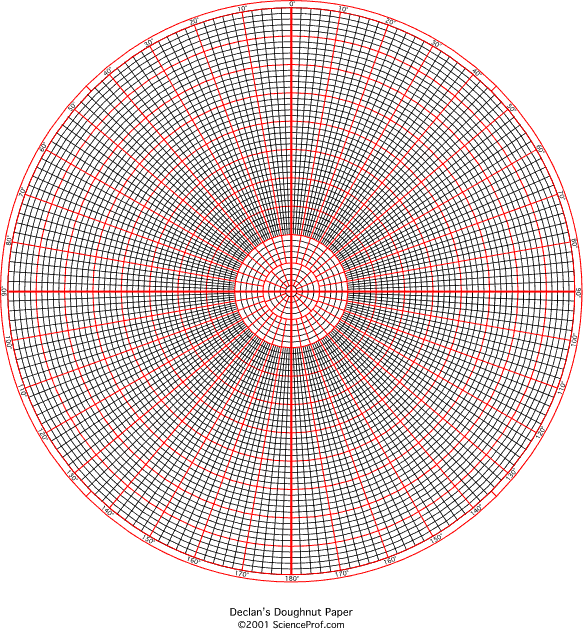
Figure 1. The Polar Grid (Click to enlarge).
The new constructions employ a polar grid of the type used for the plotting of linear rose diagrams or scatter graphs of vector data (Fig. 1). The difference between this grid and a polar stereonet such as the Lambert Projection lies in the constant spacing of the concentric circles and the arbitrary outer limit here chosen as 10 bold units.
To facilitate scaling operations, a net of 10 cm radius with concentric circles drawn bold every 1 cm and light every 2 mm is used here. (The actual units are not specified - they could be Megapascals, or pounds per square inch for stress analysis, pure numbers in the case of strain, or rates in the case of flow). Angles are marked lightly at 2-degree intervals and heavily every 10-degrees, over all but the innermost part of the grid.
The Simplest Stress Construction: Uniaxial Stress: Animated Version
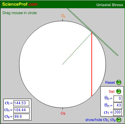
Figure 2. Animation for solving uniaxial stress problems
To begin, let us consider the simple problem of determining the total stress σt on an arbitrary inclined plane under a uniaxial principal stress, say σ1 = 200 MPa (the subscript t is used because σt refers to the total load on a plane per unit area and generally has both normal and shear stress components, σn and σs). The problem is solved by an interactive flash animation, a snapshot of which is illustrated in Fig. 2. A circle is drawn with a diameter representing 200 MPa. A bold red line represents a vertical stress vector. Solid and hashed green lines of arbitrary length represent, respectively, the normal and trace of the plane on which that stress acts. If you drag the computer mouse around the circle, the inclined plane tracks the mouse movement and the stress shown in red represents the total stress, σt, as a function of pole orientation, θn. Toggling the show/hide button reveals the normal and shear stress components which are drawn in magenta. Note that the orientation of the total stress vector in this case remains constant; only the stress magnitude changes with orientation of the plane of application. For simplicity, the maximum stress is chosen vertical in the case illustrated; other orientations are simply entered into the θ0 text field.