Results
Results of the simulations are presented in Figs. 3-6. Figure 3 shows the 3D development of the central inclusion surface during spiral formation, while Fig. 4 shows 2D movies of spiral development in the XZ, XY and YZ planes. The XZ plane is perpendicular to both the shear plane and axis of relative rotation between sphere and matrix, while the XY plane is parallel to the shear plane, and the YZ plane is perpendicular to the shear plane and parallel to the axis of relative rotation between sphere and matrix. Figure 5 compares the final rotation and non-rotation simulation geometries, and Fig. 6 shows 2D movies of serial slices through the spirals parallel to the XZ, XY and YZ planes. Results of both the rotation and non-rotation simulations are presented in these figures.
Figure 3. Movies of the non-rotation (a) and rotation (b) models of spiral formation
Movie 3a
Movie 3b
For maximum clarity, the movies show the development of the central inclusion surface only. A green marker has been added to the sphere margin to provide a visual trace of sphere rotation during the simulation. Note, this marker has been positioned on the sphere margin in all frames of the movie, and does not represent equivalent marker points within the simulation at different stages of spiral development. In the non-rotation movie, arrows indicate the sense of matrix shear. The long axes of the arrows are parallel to the orientation of the shear plane, and parallel to the orientation of the theoretically developing matrix foliation.
3D spiral development, non-rotation simulation
In the non-rotation simulation, the matrix wraps around the irrotational growing sphere, and it is this shape, in combination with the rotation of the matrix foliation about the sphere, that defines the 3D geometry of the spiral (Figs. 3a, 4d-f). Further from the sphere, the matrix is unaffected by the flow perturbation about the sphere and maintains a sub-planar geometry during the course of the simulation. The maximum perturbation of the matrix occurs in the plane through the centre of the sphere, perpendicular to the axis of relative rotation between the sphere and matrix. The perturbation decreases to zero along the axis of relative rotation as we move away from the centre of the sphere, resulting in a strongly non-cylindrical spiral geometry.
From the centre to the rim of the sphere, the central inclusion plane develops with intervals of relatively gentle curvature separated by intervals of relatively tight curvature. The reason for this is related to the repeated cycles of foliation development in the matrix. At the initiation of each new foliation, the matrix foliation is oriented at approximately 90° to the new shear plane, and is thus quickly rotated toward the shear plane. The rate of rotation slows once the matrix foliation is oriented close to the shear plane. Thus the spiral development is marked by periods of relatively rapid rotation of the foliation about the sphere, coinciding with the development of a new foliation, and periods of relatively slower rotation as the new foliation matures and is reoriented closer to the shear plane.
Figure 4. Movies showing the progressive development of spiral inclusion trails according to both the rotation and non-rotation models of spiral formation
Movie 4a
Movie 4b
Movie 4c
Movie 4d
Movie 4e
Movie 4f
Spiral development is shown in sections oriented parallel to the XZ, XY, and YZ planes. Equivalent colours represent equivalent surfaces in different sections of each simulation. Subplots show the orientation of the 2D sections with respect to the spiral. In all figures, the sphere is represented by a dashed black line.
3D spiral development, rotation simulation
As with the non-rotation simulation, the non-cylindrical spiral geometry reflects the wrapping of the matrix foliation around the growing porphyroblast, although in the rotation simulation, it is the rotation of the sphere, rather than the matrix, that is the driving force behind spiral formation. Once captured within the sphere, the foliation is progressively rotated away from the equivalent foliation in the matrix, thus forming the spiral geometry. The central inclusion surface forms a doubly curving non-cylindrical geometry, whose development can be visualised as a symmetrical pair of sheath folds. Once formed, the sheath fold is progressively rotated and stretched about the axis of relative rotation between the porphyroblast and matrix (Fig. 3b). The central surface develops relatively smoothly compared to the non-rotation simulation. The development of foliation surfaces that were originally oriented off-centre with respect to the sphere can be visualised as the progressive rotation and elongation of a single sheath fold (Fig. 4a). The part of the spiral further from the ‘sheath fold’ tip has a more open geometry due to the wrapping of the matrix foliation about the growing sphere.
3D spiral geometry
The final 3D spiral geometries are summarised in Fig. 5, while movies showing 2D sections through the spirals are shown in Fig. 6. The rotation and non-rotation spirals are similar, and comparable to spiral geometries published in previous studies (e.g. Gray & Busa, 1994). As described above, the central inclusion surface of both simulations is a doubly curving non-cylindrical geometry, and can be visualised as a symmetrical pair of oppositely facing sheath folds. Inclusion trail surfaces initially positioned off-centre with respect to the respective spheres developed geometries that resemble single sheath folds. Surfaces originally positioned at progressively greater distances from the porphyroblast centre develop sheath fold geometries that are narrower and less elongate compared with those originally positioned close to the sphere centre (e.g. compare Fig. 5e,f with Fig. 5g,h). Cross sections through the sheath folds reveal distinctive closed loop patterns (Fig. 6).
Figure 5. Comparison of the 3D geometry of the rotation and non-rotation spiral simulations
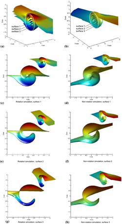
(a) and (b) show the rotation and non-rotation simulations respectively, and the porphyroblast is outlined in white. The inclusion surfaces individually labelled on (a) and (b) are shown separately in Figures (c)-(h) to illustrate the varied geometry of surfaces located at increasing distances from the porphyroblast centre. The rotation and non-rotation simulations are viewed from opposite directions in order to give the same shear sense and enable comparison of the two sets of geometries. Note, the dark wrinkled areas on Figs (d) and (f) are due to the limits of resolution of the simulation, and are not real features of the spiral geometry.
A useful way to visualise the 3D spiral geometry is to use the analogy of a breaking wave. The matrix foliation is represented by the ocean surface, upon which a wave has formed. The wave has a limited lateral extent, equal to little more than the height of the wave itself. The height of the wave is greatest in the central part, and diminishes steadily toward the wave margins. The leading edge of the wave is also most advanced in the central section, and diminishes to zero at the wave margins. As the amount of spiral curvature increases, the tip of the wave breaks down toward the hollow in front of the wave, but instead of breaking into the surf below, the leading tip curls upward (against gravity!) and back in on itself (e.g. Fig. 5). We must invert the analogy to visualise the development of inclusion surfaces that form in the lower half of the sphere (e.g. Fig. 5e,f). This analogy helps to visualise the final simulation geometry, although it does not represent the process of spiral formation.
Figure 6. Serial 2D slices through the final spiral geometries of the rotation and non-rotation simulations
Movie 6a
Movie 6b
Movie 6c
Movie 6d
Movie 6e
Movie 6f
The spiral geometry is shown in sections parallel to the XZ, XY and YZ planes. Sections have been cut parallel to the shear plane (XY plane), perpendicular to the shear plane and parallel to the axis of relative rotation between sphere and matrix (YZ plane), and perpendicular to both the shear plane and axis of relative rotation between sphere and matrix (XZ plane). Subplots show the orientation of the 2D sections with respect to the spiral.
The effect of theta on spiral geometry
In terms of the rotation model, the final inclusion trail geometry is greatly dependent on the angle between the pre-deformation foliation and the shear plane (we call this angle ‘theta’). This is because the asymmetry of inclusion trail curvature is controlled by the relative rate of rotation of the sphere and matrix, which in turn is related to the angle between the shear plane and the matrix foliation adjacent to the sphere. For instance, when theta is greater than 135° or less than 45°, the sphere rotates toward the shear plane more rapidly than the matrix, whereas for theta values of between 45° and 135°, the matrix rotates toward the shear plane at a greater rate than the sphere. Simple shear deformation acts to rotate the matrix foliation toward the shear plane and thus progressively reduce the theta value. This means that for simulations with an initial theta of >135°, reversals in inclusion trail asymmetry occur as the foliation is rotated through the crucial theta values of 135° and 45°. It is at these points in the simulation that a switch occurs in the relative rates of rotation of the sphere and matrix. This is illustrated in the theta=160° movie, in which two switches in curvature asymmetry are clearly observed (Fig. 7g). On the basis of these patterns, Masuda & Mochizuki (1989) distinguished three types of inclusion trail patterns: single rotation types (theta <45°), which record consistent asymmetry from core to rim, double rotation types (45°<theta<135°), which record one reversal of curvature from core to rim, and triple rotation types (theta>135°), which record two reversals in asymmetry.
Figure 7. The effect of varying theta (angle between pre-deformation matrix foliation and shear plane) on spiral inclusion trail geometry
Movie 7a
Movie 7b
Movie 7c
Movie 7d
Movie 7e
Movie 7f
Movie 7g
Movie 7h
Movies show spiral development in the XZ plane. All simulations involved simple shear deformation of the matrix and full coupling between sphere and matrix.
In terms of the non-rotation model, it is possible to create almost unlimited variations of the geometry presented in Fig. 3 by varying the value of theta for each foliation developed during the course of the simulation. However, such an exercise is of limited use, and we have chosen to set theta at 90° for the non-rotation simulation, in accordance with the non-rotation model of Bell (1985) and Bell & Johnson (1989).
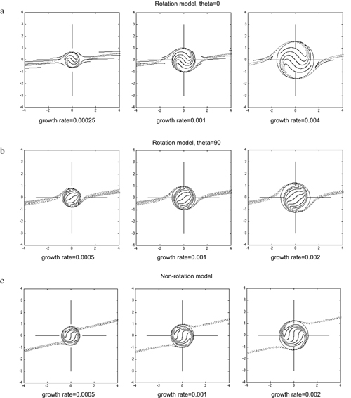
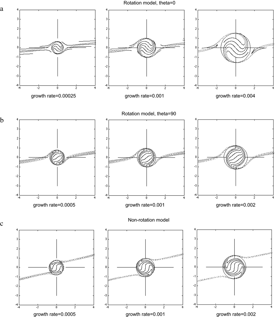
The effect of growth rate on spiral geometry
Variation in the rate of sphere growth has no effect on 3D spiral geometry, although the overall size of the spiral is larger in simulations with a higher growth rate (Fig. 8). The reason for this is that although a sphere with a faster growth rate is larger at any given point in time compared with its slower growing equivalent, the ratio of the radiuses of the two spheres is constant during the course of the simulation. To illustrate this point, consider the growth of two spheres, A and B, of growth rates ΔV and ΔV.α respectively, where ΔV is the change in sphere volume with each time step of the simulation, and α is a constant (e.g. 3) that indicates a faster growth rate for sphere B. We can determine the radius of each sphere (r), after a given interval of time (t), using the relationship between the volume and radius of a sphere (V=4πr3). For sphere A, the volume after time t is equal to and the radius is equal to

The equivalent expression for sphere B is

At any given stage in the simulation, the radius of sphere B is greater than that of sphere A by the ratio of 3√α, which is a constant. Thus, for sphere growth that involves volume increase at a constant rate, identical 3D inclusion patterns develop, although at different scales, irrespective of growth rate.
Figure 8. The spiral geometries that result from simulations with varying rates of sphere growth
The growth rate refers to the increase in unit volume during each calculation step in the simulations. All figures are XZ sections.
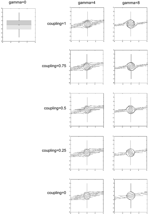
The effect of coupling on spiral geometry
The numerical code used in this study does not describe the physical nature of the coupling between sphere and matrix. Instead, the degree of coupling is approximated by the parameter k (Bjornerud & Zhang, 1994), which varies from 0 (no coupling) to 1 (full coupling). The amount of sphere rotation at each time step in the simulation (calculated according to conditions of full coupling between the sphere and matrix) is multiplied by k to approximate the rotation of the sphere at a desired value of coupling. The component of matrix shear resulting from the effect of sphere rotation is also multiplied by k.
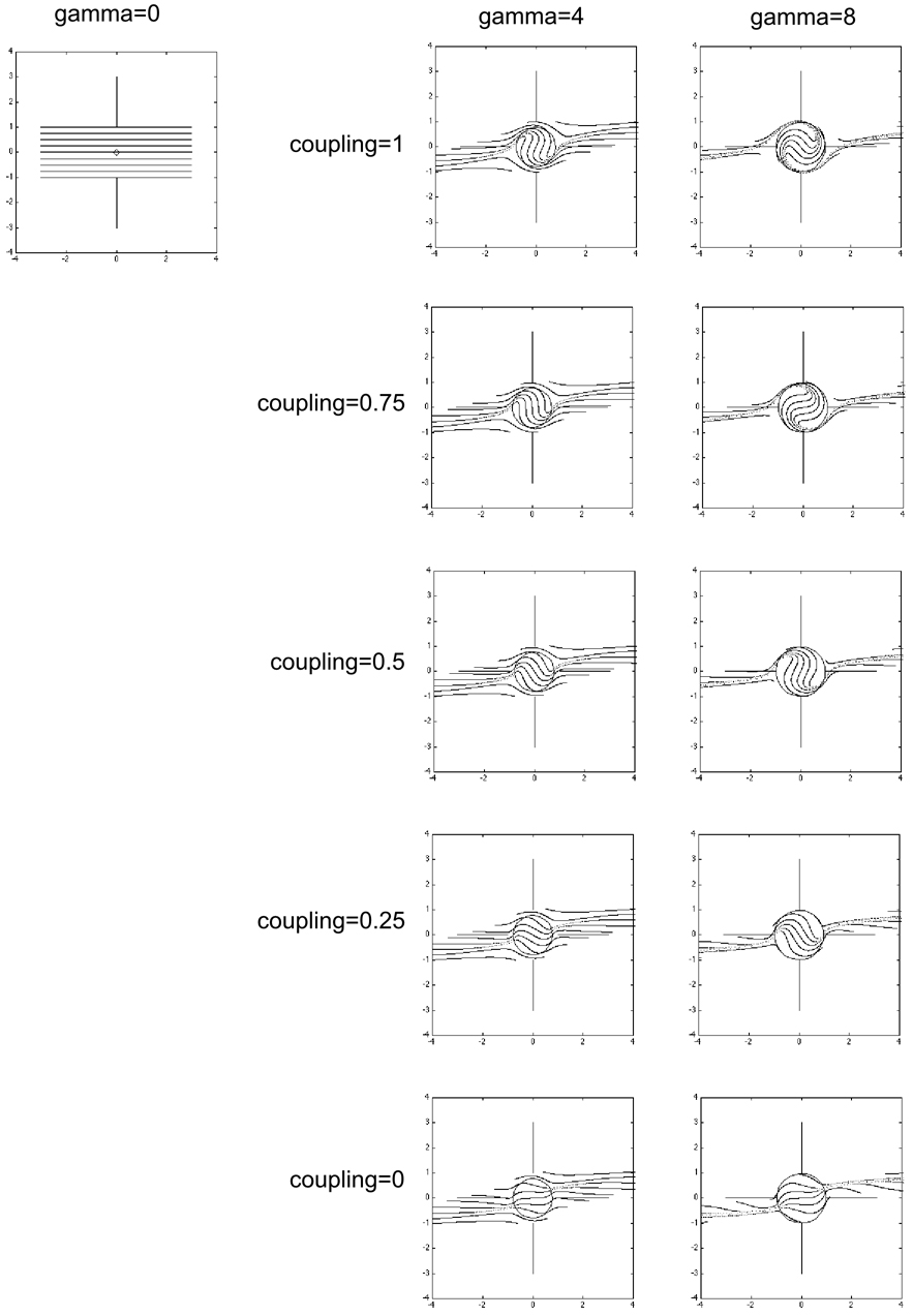
In terms of the rotation model, reduced coupling between the sphere and matrix results in a decrease in the rate of sphere rotation, and accordingly a reduction in the total inclusion trail curvature (Fig. 9; see also fig. 1 from Bjornerud & Zhang, 1994). For coupling values of <0.25, the geometry of the inclusion trails departs from the normal spiral shape, and this distinctive geometry, if observed in rocks, may be useful as an indicator of weak coupling between porphyroblast and matrix. For coupling values of >0.25, spiral geometry is not a useful indicator of the degree of coupling, as all simulations with coupling >0.25 produce spiral-like geometries. For example, in Fig. 9, it is difficult to distinguish the spiral that formed with coupling=0.5, gamma=8, from that which formed under conditions of coupling=1, Gamma=4. Although the coupling=0 inclusion pattern differs from typical spiral geometry, it is still possible to produce a spiral geometry with coupling=0 if the simulation involves multiple overprinting foliations.
Figure 9. The effect on spiral geometry of varying the degree of coupling between the sphere and matrix
All figures are XZ sections. All simulations involved simple shear deformation of the matrix.
The effect of pure shear deformation on spiral geometry
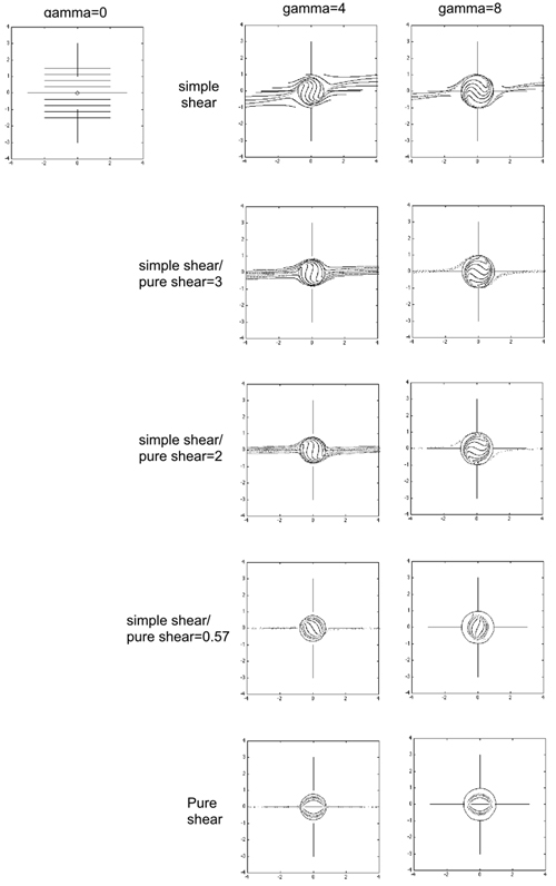
As the pure shear component of matrix deformation is increased, the rate of sphere rotation decreases, and the amount of inclusion trail curvature recorded within the sphere is also reduced (Fig. 10). The matrix foliation is also subjected to greater flattening and extension within the XY plane. This creates problems with the simulation, as marker points within the matrix rapidly move toward the simulation boundaries (e.g. Fig. 10). It is apparent from Fig. 10 that a large component of simple shear is required to generate a spiral geometry. Simple shear deformation is indeed described by the rotation model, and the non-rotation model also details foliation curvature in zones of non-coaxial deformation, although in contrast to the rotation model, these zones are partitioned into anastomosing seams adjacent to the porphyroblast.
Figure 10. The effect on spiral geometry of varying the proportion of simple and pure shear deformation within the matrix
All figures are XZ sections. In all simulations, the sphere was fully coupled to the matrix.
Comparison of the rotation and non-rotation simulations
Although the results of the rotation and non-rotation simulations are very similar (e.g. Fig. 5), we are able to identify four differences in the 3D geometry of the two simulations. These are: smoothness of spiral curvature, spacing of foliation planes, alignment of individual foliation planes within the matrix either side of the porphyroblast, and spiral asymmetry with respect to matrix shear sense. The degree of similarity between the two sets of simulations is important, as 3D spiral geometry has previously been proposed as a criterion for distinguishing between the competing models in rocks (e.g. Williams & Jiang, 1999). We explore this topic more fully in a separate paper arising from the data presented in this study (Stallard et al., in press).
Comparison with previous studies
The spiral simulations presented in this study are broadly comparable to the various theoretical, mechanical and numerical models of spiral geometry published previously by Powell & Treagus (1967, 1970), Masuda & Mochizuki (1989), Gray & Busa (1994), and Schoneveld (1977), and with the sections through real garnets published by Johnson (1993a). However, the simulations are different to those presented by Williams & Jiang (1999) as representative of spirals produced by the non-rotation model. Williams & Jiang based their interpretation on Johnson’s (1993b) description of the non-rotation hypothesis, and concluded that the 3D spiral geometry produced by the non-rotation model is different to the geometry produced by the rotation model. The results of this study are contrary to the conclusions of Williams and Jiang, and the implications of this are discussed in a separate paper (Stallard et al., submitted).