The effect of growth rate on spiral geometry

Variation in the rate of sphere growth has no effect on 3D spiral geometry, although the overall size of the spiral is larger in simulations with a higher growth rate (Fig. 8). The reason for this is that although a sphere with a faster growth rate is larger at any given point in time compared with its slower growing equivalent, the ratio of the radiuses of the two spheres is constant during the course of the simulation. To illustrate this point, consider the growth of two spheres, A and B, of growth rates ΔV and ΔV.α respectively, where ΔV is the change in sphere volume with each time step of the simulation, and α is a constant (e.g. 3) that indicates a faster growth rate for sphere B. We can determine the radius of each sphere (r), after a given interval of time (t), using the relationship between the volume and radius of a sphere (V=4πr³). For sphere A, the volume after time t is equal to and the radius is equal to

The equivalent expression for sphere B is

At any given stage in the simulation, the radius of sphere B is greater than that of sphere A by the ratio of ³√α, which is a constant. Thus, for sphere growth that involves volume increase at a constant rate, identical 3D inclusion patterns develop, although at different scales, irrespective of growth rate.

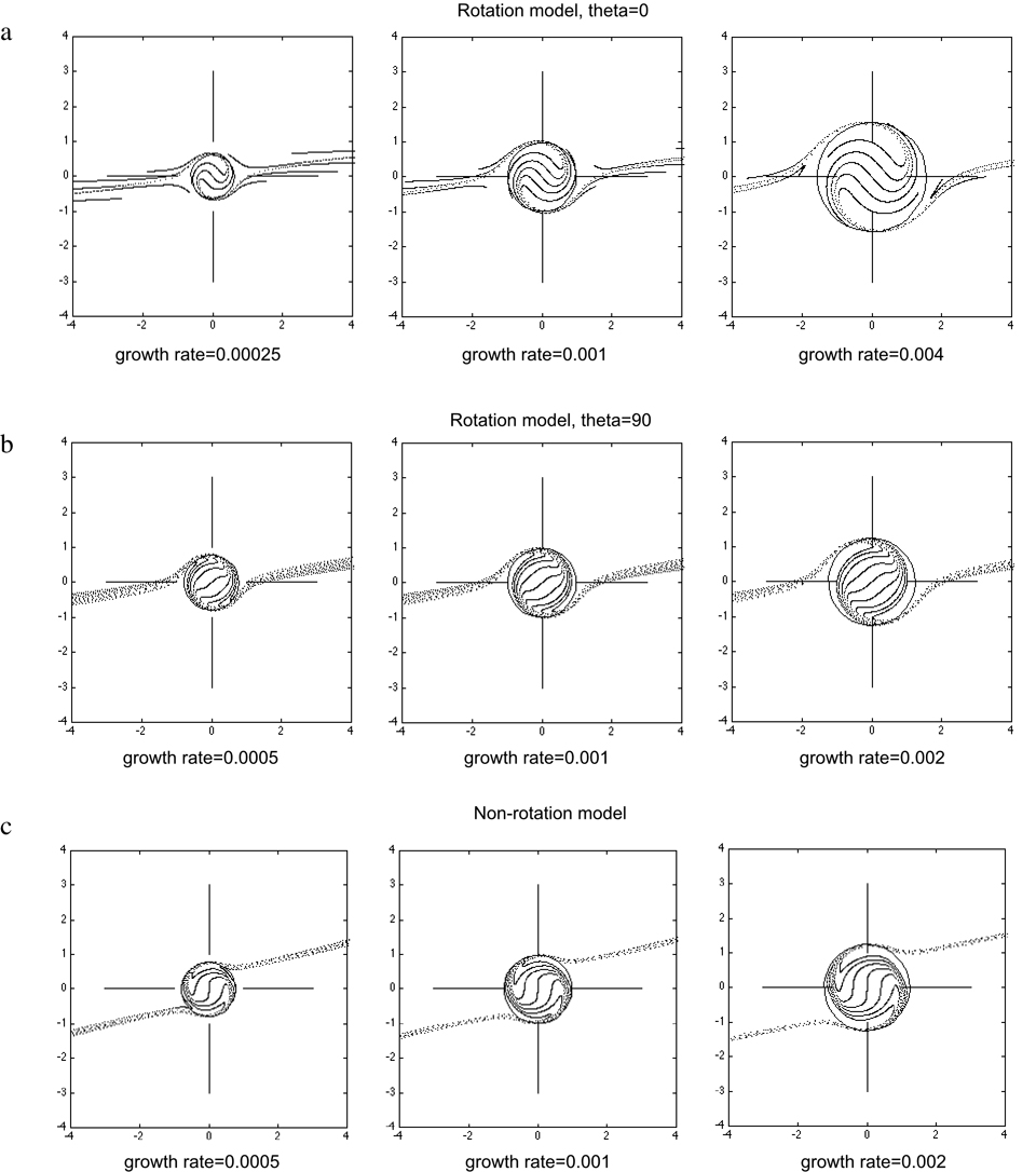Figure 8. These figures show the spiral geometries that result from simulations with varying rates of sphere growth. The growth rate refers to the increase in unit volume during each calculation step in the simulations. All figures are XZ sections. (Click for enlargement)

The effect of coupling on spiral geometry

The numerical code used in this study does not describe the physical nature of the coupling between sphere and matrix. Instead, the degree of coupling is approximated by the parameter k (Bjornerud & Zhang, 1994), which varies from 0 (no coupling) to 1 (full coupling). The amount of sphere rotation at each time step in the simulation (calculated according to conditions of full coupling between the sphere and matrix) is multiplied by k to approximate the rotation of the sphere at a desired value of coupling. The component of matrix shear resulting from the effect of sphere rotation is also multiplied by k.
In terms of the rotation model, reduced coupling between the sphere and matrix results in a decrease in the rate of sphere rotation, and accordingly a reduction in the total inclusion trail curvature (Fig. 9; see also fig. 1 from Bjornerud & Zhang, 1994). For coupling values of <0.25, the geometry of the inclusion trails departs from the normal spiral shape, and this distinctive geometry, if observed in rocks, may be useful as an indicator of weak coupling between porphyroblast and matrix. For coupling values of >0.25, spiral geometry is not a useful indicator of the degree of coupling, as all simulations with coupling >0.25 produce spiral-like geometries. For example, in Fig. 9, it is difficult to distinguish the spiral that formed with coupling=0.5, gamma=8, from that which formed under conditions of coupling=1, Gamma=4. Although the coupling=0 inclusion pattern differs from typical spiral geometry, it is still possible to produce a spiral geometry with coupling=0 if the simulation involves multiple overprinting foliations.

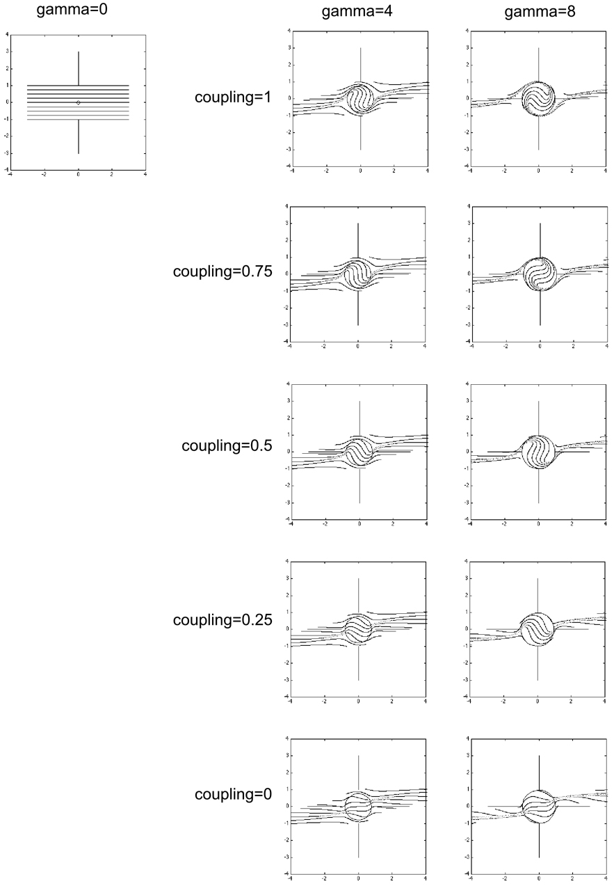Figure 9. These figures show the effect on spiral geometry of varying the degree of coupling between the sphere and matrix. All figures are XZ sections. All simulations involved simple shear deformation of the matrix. (Click for enlargement)

The effect of pure shear deformation on spiral geometry

As the pure shear component of matrix deformation is increased, the rate of sphere rotation decreases, and the amount of inclusion trail curvature recorded within the sphere is also reduced (Fig. 10). The matrix foliation is also subjected to greater flattening and extension within the XY plane. This creates problems with the simulation, as marker points within the matrix rapidly move toward the simulation boundaries (e.g. Fig. 10). It is apparent from Fig. 10 that a large component of simple shear is required to generate a spiral geometry. Simple shear deformation is indeed described by the rotation model, and the non-rotation model also details foliation curvature in zones of non-coaxial deformation, although in contrast to the rotation model, these zones are partitioned into anastomosing seams adjacent to the porphyroblast.

Figure 10. These figures show the effect on spiral geometry of varying the proportion of simple and pure shear deformation within the matrix. All figures are XZ sections. In all simulations, the sphere was fully coupled to the matrix. (Click for enlargement)

Comparison of the rotation and non-rotation simulations

Although the results of the rotation and non-rotation simulations are very similar (e.g. Fig. 5), we are able to identify four differences in the 3D geometry of the two simulations. These are: smoothness of spiral curvature, spacing of foliation planes, alignment of individual foliation planes within the matrix either side of the porphyroblast, and spiral asymmetry with respect to matrix shear sense. The degree of similarity between the two sets of simulations is important, as 3D spiral geometry has previously been proposed as a criterion for distinguishing between the competing models in rocks (e.g. Williams & Jiang, 1999). We explore this topic more fully in a separate paper arising from the data presented in this study (Stallard et al., in press).

Comparison with previous studies

The spiral simulations presented in this study are broadly comparable to the various theoretical, mechanical and numerical models of spiral geometry published previously by Powell & Treagus (1967, 1970), Masuda & Mochizuki (1989), Gray & Busa (1994), and Schoneveld (1977), and with the sections through real garnets published by Johnson (1993a). However, the simulations are different to those presented by Williams & Jiang (1999) as representative of spirals produced by the non-rotation model. Williams & Jiang based their interpretation on Johnson’s (1993b) description of the non-rotation hypothesis, and concluded that the 3D spiral geometry produced by the non-rotation model is different to the geometry produced by the rotation model. The results of this study are contrary to the conclusions of Williams and Jiang, and the implications of this are discussed in a separate paper (Stallard et al., submitted).