3D spiral geometry

The final 3D spiral geometries are summarised in Fig. 5, while movies showing 2D sections through the spirals are shown in Fig. 6. The rotation and non-rotation spirals are similar, and comparable to spiral geometries published in previous studies (e.g. Gray & Busa, 1994). As described above, the central inclusion surface of both simulations is a doubly curving non-cylindrical geometry, and can be visualised as a symmetrical pair of oppositely facing sheath folds. Inclusion trail surfaces initially positioned off-centre with respect to the respective spheres developed geometries that resemble single sheath folds. Surfaces originally positioned at progressively greater distances from the porphyroblast centre develop sheath fold geometries that are narrower and less elongate compared with those originally positioned close to the sphere centre (e.g. compare Fig. 5e,f with Fig. 5g,h). Cross sections through the sheath folds reveal distinctive closed loop patterns (Fig. 6).

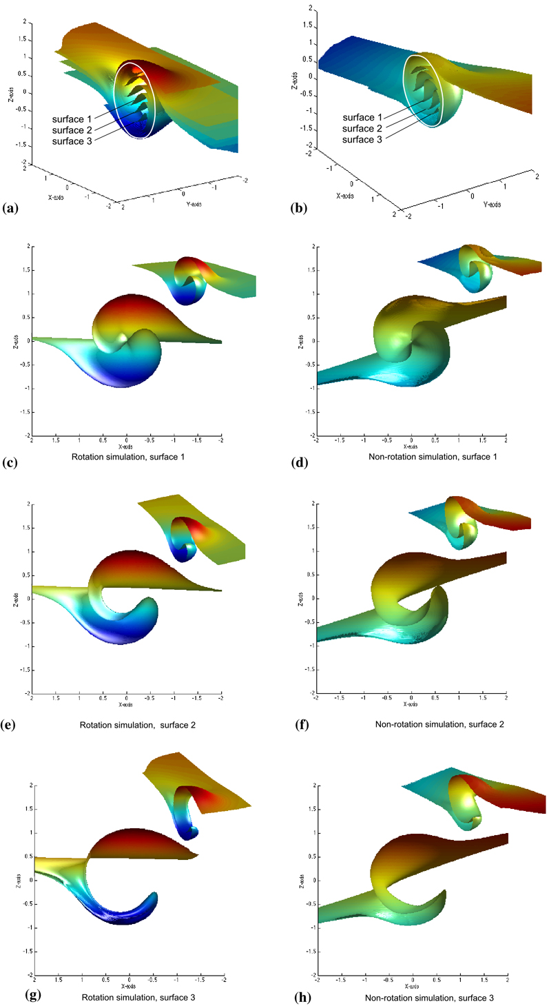Figure 5. Comparison of the 3D geometry of the rotation and non-rotation spiral simulations. (a) and (b) show the rotation and non-rotation simulations respectively, and the porphyroblast is outlined in white. The inclusion surfaces individually labelled on (a) and (b) are shown separately in Figures (c)-(h) to illustrate the varied geometry of surfaces located at increasing distances from the porphyroblast centre. The rotation and non-rotation simulations are viewed from opposite directions in order to give the same shear sense and enable comparison of the two sets of geometries. Note, the dark wrinkled areas on Figs (d) and (f) are due to the limits of resolution of the simulation, and are not real features of the spiral geometry. (Click for enlargement)

A useful way to visualise the 3D spiral geometry is to use the analogy of a breaking wave. The matrix foliation is represented by the ocean surface, upon which a wave has formed. The wave has a limited lateral extent, equal to little more than the height of the wave itself. The height of the wave is greatest in the central part, and diminishes steadily toward the wave margins. The leading edge of the wave is also most advanced in the central section, and diminishes to zero at the wave margins. As the amount of spiral curvature increases, the tip of the wave breaks down toward the hollow in front of the wave, but instead of breaking into the surf below, the leading tip curls upward (against gravity!) and back in on itself (e.g. Fig. 5). We must invert the analogy to visualise the development of inclusion surfaces that form in the lower half of the sphere (e.g. Fig. 5e,f). This analogy helps to visualise the final simulation geometry, although it does not represent the process of spiral formation.

The effect of theta on spiral geometry

In terms of the rotation model, the final inclusion trail geometry is greatly dependent on the angle between the pre-deformation foliation and the shear plane (we call this angle ‘theta’). This is because the asymmetry of inclusion trail curvature is controlled by the relative rate of rotation of the sphere and matrix, which in turn is related to the angle between the shear plane and the matrix foliation adjacent to the sphere. For instance, when theta is greater than 135° or less than 45°, the sphere rotates toward the shear plane more rapidly than the matrix, whereas for theta values of between 45° and 135°, the matrix rotates toward the shear plane at a greater rate than the sphere. Simple shear deformation acts to rotate the matrix foliation toward the shear plane and thus progressively reduce the theta value. This means that for simulations with an initial theta of >135°, reversals in inclusion trail asymmetry occur as the foliation is rotated through the crucial theta values of 135° and 45°. It is at these points in the simulation that a switch occurs in the relative rates of rotation of the sphere and matrix. This is illustrated in the theta=160° movie, in which two switches in curvature asymmetry are clearly observed (Fig. 7g). On the basis of these patterns, Masuda & Mochizuki (1989) distinguished three types of inclusion trail patterns: single rotation types (theta <45°), which record consistent asymmetry from core to rim, double rotation types (45°<theta<135°), which record one reversal of curvature from core to rim, and triple rotation types (theta>135°), which record two reversals in asymmetry.

In terms of the non-rotation model, it is possible to create almost unlimited variations of the geometry presented in Fig. 3 by varying the value of theta for each foliation developed during the course of the simulation. However, such an exercise is of limited use, and we have chosen to set theta at 90° for the non-rotation simulation, in accordance with the non-rotation model of Bell (1985) and Bell & Johnson (1989).