Crustal Structure of South India From Aeromagnetic Data.

Introduction

Aeromagnetic surveys over parts of India have been conducted as part of a National Program organized by the Geological Survey of India (GSI) with professional and technical assistance from the National Remote Sensing Agency (NRSA). The survey results have been published in the form of total intensity contour maps in degree sheet format without incorporating corrections due to main field variations of the Earth. Over South India Reddy et al.. (1988) have published valuable results up to 12 degrees north and under Project Vasundhara (1994) Geological Survey of India have utilized the aeromagnetic data up to 14∞N for their interpretation and only published the trends of the anomalies. Bahulayen (1997) has published a map of the region up to 14∞N incorporating corrections for the main geomagnetic field. Aeromagnetic degree sheet maps up to 17o N were re-digitized manually at 6” (10 km) interval, processed and the results published by Harikumar et al.. (2000) and Rajaram et al.. (2001), mainly for long wavelength studies. In this paper the authors were able to delineate the orthopyroxine isograd, demarcating NW-SE trends to the north and E-W trends to the south of it. The source rock of magnetic anomalies was charnockites in the Southern Granulite Terrain and mainly intrusives/iron ore bodies in the Dharwar craton. From the analysis of fine grid aeromagnetic data in the Central Indian region, Rajaram and Anand (2003) identified a hitherto unknown shear, called the Main Peninsular Shear.

The data grid spacing has a crucial effect on the nature of the map prepared. Maps made with small grid spacing can delineate finer details, while those with larger grid spacing represent larger wavelengths corresponding to broader, deeper features. With the availability of machine digitization it is possible to have these analog degree sheets in digital format that can be used for analyzing these maps critically to derive more useful information regarding structural trends, position of faults, distribution of shallow or deep crystalline basement, occurrence of volcanic rocks within sedimentary region etc. The study of the spatial distribution of magnetic field facilitates the understanding of the regional as well as the global tectonic features. To have an understanding of the regional features, the maps have to be digitized at coarse interval and to throw light on finer details the sampling interval should be as small as possible. In this paper we are dealing with aeromagnetic data up to 180 N digitized closely along contours to throw light on the shallow as well as deeper features.

Geology and Tectonics

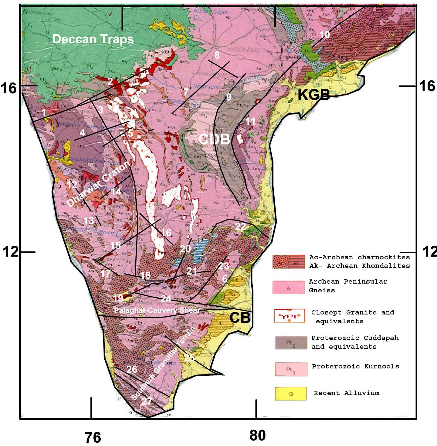
The region under study is composed of Dharwar block bounded to the south by the Southern Granulite Terrain, to the east by the Eastern Ghat Mobile Belt (EGMB) and to the northwest by the Deccan Trap flows. Figure 1 depicts the Geology and Tectonic of Peninsular India up to 180 N. The Dharawar craton comprises an upper crust of Greenstone-Granite Domain, cratonized more or less by the Early Proterozoic that continued to evolve in the whole of Proterozoic (Mahadevan, 2003). The NS trending Closepet granite is a conspicuous feature in the Dharwar block. The Dharwar block can be divided further into an eastern and western Dharwar blocks with Chitradurga Schist belt (Anand and Rajaram 2002, Project Vasundra, 1994) as the dividing line while others believe Closept Granite to be the dividing line (Swami Nath et al., 1976, Subrahmanayam and Verma, 1982). The Eastern block is dominated by the Kolar type schist belt (aurifrous ~ 2.5 Ga) while the western block is composed of Dharwar type schist belt (large schist belt ~ 3.0 Ga). The most characteristic feature of the Archean cover sequence of the Dharwar craton is their arcuate NS trend with convexity towards east. The western Dharwar craton, is a typical low-grade terrain characterized by mature sediment dominated greenstone belt of Dharwar type. Banded iron formations are found associated with the Bababudan and Kudremukh belt in addition to Sandur and Goa basins. The Eastern Dharwar block is typified by volcanic dominated greenstone belt (Keewatian type) characterized by low-pressure metamorphism. The prominent schist belts trending NNW-SSE are volcanogenic and are known for their gold mineralization. The most important linear feature of the region includes NNW trending Chitradurga Boundary Shear (3) (CBS). ENE trends include Krishna river fault (2), Dharma-Tungabadhra lineament (4), Kumudavati-Narihalla lineament (5) etc. Isotopic age studies using K-Ar, Rb-Sr and Pb methods placed the western Dharwar craton to be older than the Eastern block (Project Vasundhara, 1994).

The Southern Granulite Terrain (SGT), extending from 8 to 13o N latitude (up to Orthopyroxene isograd), of India is one of the few terrains in the world that has preserved Archean crust with extensive granulites, believed to be of lower-crustal origin. The region is a mosaic of high-grade granulite massifs with shear zones in between. The Dharwar craton is separated from the SGT by two prominent shear zones known as the Moyar-Bhavani shear zone and Palaghat-Cauvery shear zone, a transition zone marked by gradation in meatmorphism from gneisses in the north to charnockite in the south. There is a marked change in the structural trend from the dominant NS in the Dharwar block to EW in the SGT, which distinguish SGT from the Dharwar craton. The SGT is divided into three major blocks. The northern granulite block occupies the area between the Dharwar craton and the Palaghat-Cauvery shear zone and defines the transition between the low and high grade terrains ( ~ 2.5 Ga). The region between Palaghat-Cauvey shear zone and Achankovil shear zone is the Southern Granulite block ( 0.5 – 0.7 Ga) including most of the highlands. To the south of Achankovil shear zone (26) is the Kerala Khondalite block, a seat of meta-sedimentary granulites. The SGT is composed of amphibolite facies gneiss and supracrustal rocks in addition to charnockites, mafic granulites and khondalites (GSI, 2000). Radiometric dates of these lithilogic units vary between 3000 to 2000 Ma (Sarkar, 2001). The younger granites in this terrain are of Late Proterozoic age. The structural trend, south of Achankovil shear, the Khondalite belt of southern Kerala, is NW-SE. The terrain in SGT is traversed by fairly dense network of NW and NE trending lineaments. The WNW-ESE trending lineaments include Moyar Fault (18), Cauvery fault (24), Vaigai river fault (25); NW-SE trending Achankovil (26), Tenmalai fault (27); NNE-SSW trending Metur East fault (20) and NE trending Bhavani lineament (19) are some of the very prominent discontinuities which have affected all the basement elements of the terrain.

The crescent shaped Proterozoic Cuddapah basin, occurs on the eastern side of the Dharwar block. Two litho-stratigraphic groups, each with distinctive rock assemblages and ages, constitute the basin. The older Cuddapah super group occupying the entire basin is overlain by Kurnool group in the western and northeastern part. The Cuddapah rocks contain extensive dolerite sills and dykes and basaltic flows in the south-western part of the basin. The volcano-sedimentary dominated Nellore type schist belt forms a major thrust along the eastern margin of the Proterozoic Cuddapah basin. To the east of it is the Eastern Ghat Mobile Belt, a highly deformed terrain with lithological assemblages varying from Archean to recent. The basement constitutes of mainly Proterozoic highgrade gneiss-granulites consisting of charnockites, khondalites and high grade gneiss (GSI,2000) whose structural trend is NE-SW. EGMB can be differentiated from SGT by its intense deformation, characteristic NE-SW strike, abundance of Khondalites and intermingling of charnockites and khondalites and abundance of manganese formations(Sarkar, 2001). This mobile belt has undergone polyphase deformation and metamorphism.

Recent alluvial sediments form long coastal strips at the periphery of the Peninsular shield. These pericratonic pull-apart sedimentary basins (Prabhakar and Zutshi, 1993) are broader on the east coast compared to west probably due to the drainage from the large number of east flowing rivers. The sedimentary basins in the study region include the Cauvery, Palar-Pennar and Krishna-Godavari basin along the east coast of India. The NE-SW trending east coast basins formed as a result of the breakup of India from Gondwanaland, are oil bearing. The east coast basins are floored by attenuated continental crust and are characterized by parallel fault-bounded horsts and graben along the NE-SW EGMB trend. These faults appear to have evolved in a divergent setting when India separated from Antarctica in the Mesozoic.

The known faults and shears of the Peninsular shield closely follows the pattern of major rivers. The Moyar-Bhavani, Vaigai and Cauvery shears are typical examples in the SGT. Major faults/lineaments in the Dharwar craton like Krishna, Tunga-Badhra, Pennar, Bhima etc are associated with known rivers.

Aeromagnetic Map Analysis

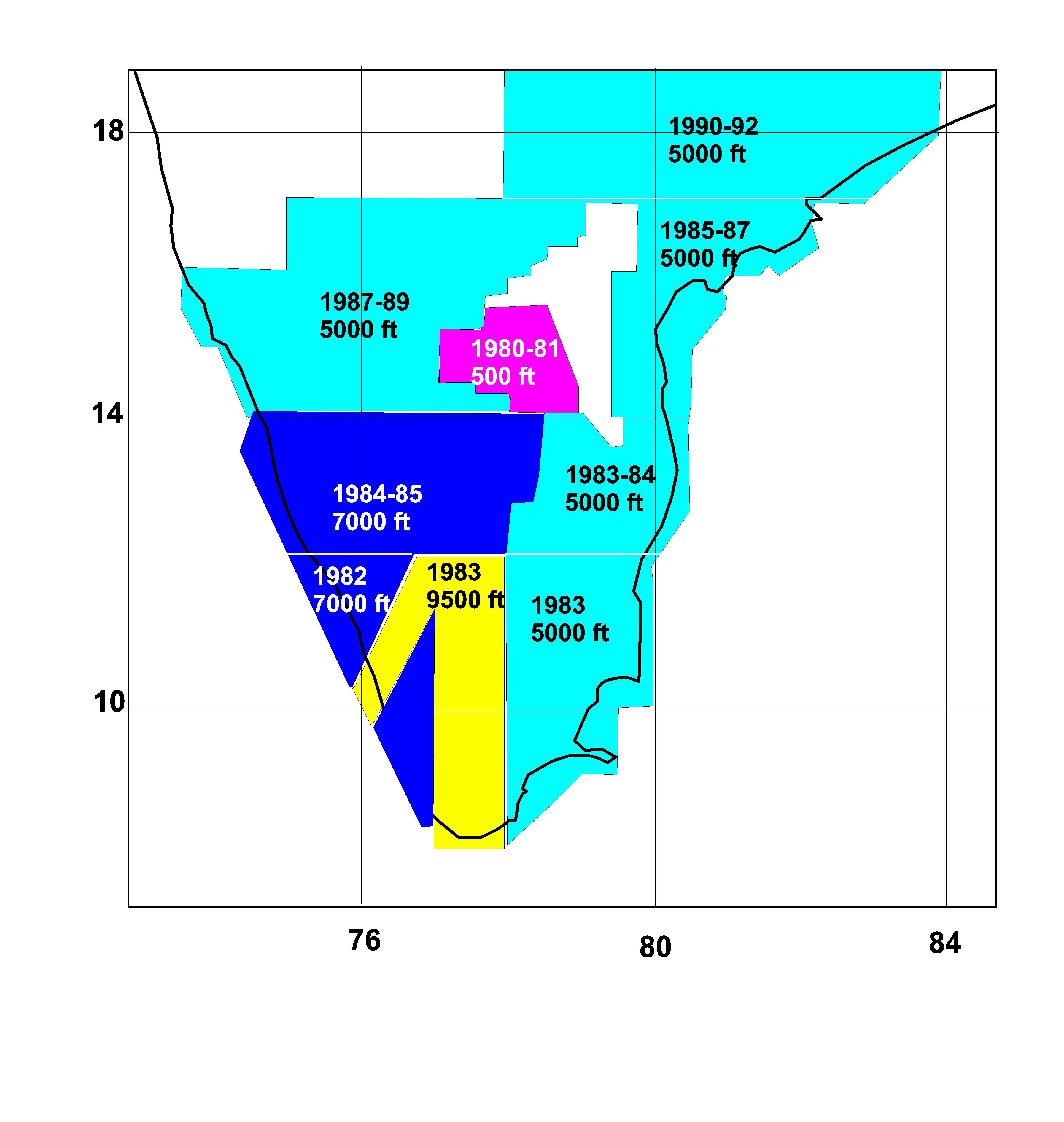
Aeromagnetic surveys over the peninsular shield were conducted in distinct epoch and altitude ranges. Figure 2 demonstrates the altitude and epoch of the aeromagnetic data collection in our region of study. In the eastern part and parts of Northern Karnataka the data are collected at an altitude of 5000ft (1515m). In the rest of the western part of the Peninsula, the data is collected at 7000ft (2121m) except in a narrow region in the centre, where the flight altitude is 9500ft (2850m), to clear high topography. The flight lines in the region where the flight altitude is 7000ft are N25°E-S25°W and for the rest of the region, the flight lines are N-S. The line spacing for all these blocks was maintained at 4km, except for the drape survey over Cuddapah basin (altitude 500’) covered under Operation Hard Rock (OHR) where, the line spacing varied from 500 meters to 1 km. It thus becomes inevitable to reduce the data to a common barometric altitude to obtain an overall idea of the magnetic response of the geological terrain in general. The catalogue published by Geological Survey of India (1995) includes details about the aeromagnetic data. There however exists a data gap, as degree sheets were not available over the Cuddapah basin. We have incorporated ground magnetic data over this basin, collected at 10km interval by Indian Institute of Geomagnetism (IIG) to fill this gap in the aeromagnetic data. Rajaram et. al (2000) noted that most of the long wavelength features at aeromagnetic height, redigitized at 6’ interval, are also evident on ground data collected at 10km interval.

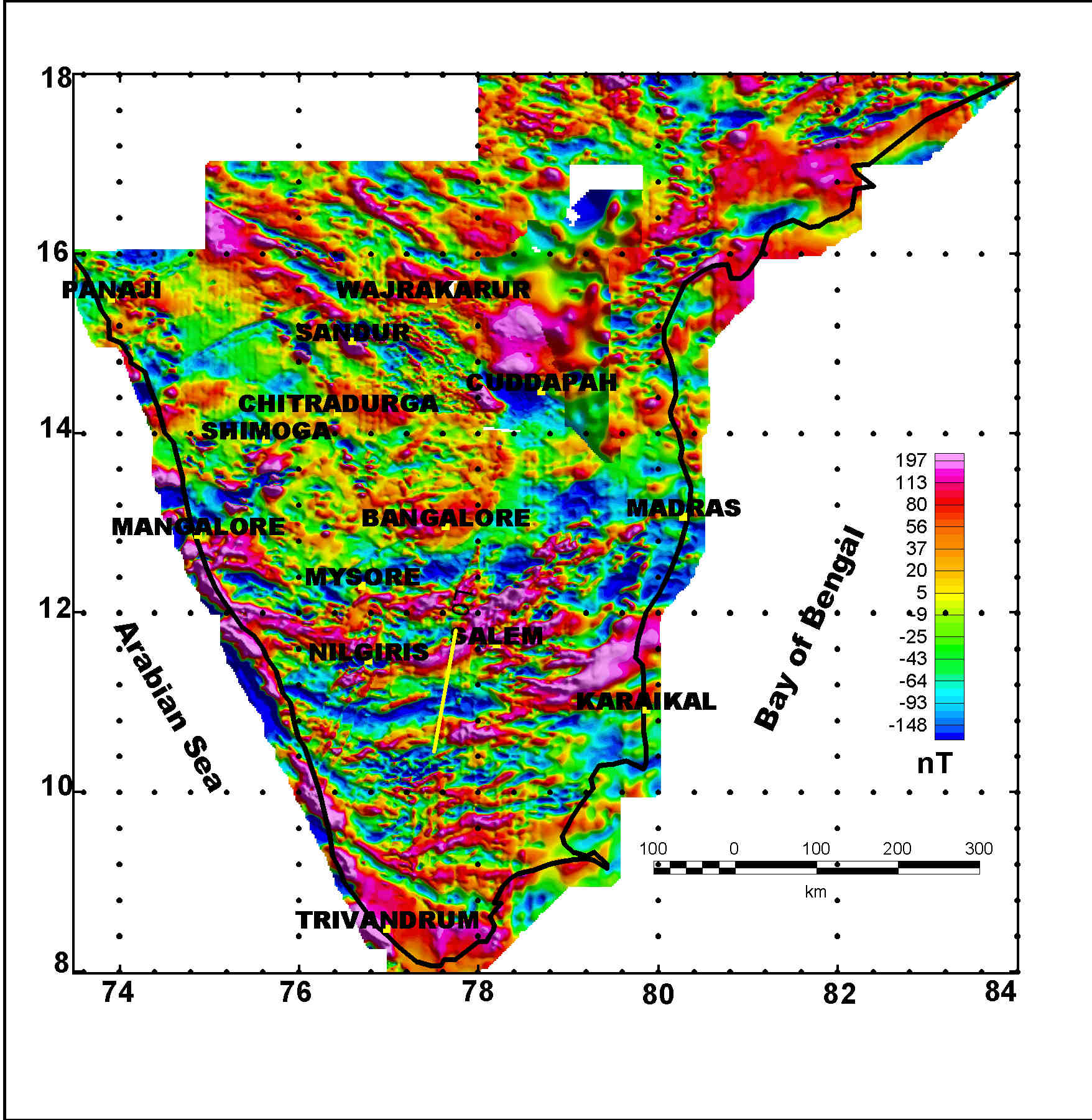
The degree sheet maps were machine digitized along contours. The observed digital aeromagnetic data for each block is corrected to remove the main field contribution using the appropriate IGRF models; thus we had to use the IGRF models 1980 and 1985, with the model being interpolated to the appropriate date and the altitude of observation. The data were then re-gird at 2km interval. The IGRF removed data in the different blocks are at different elevations therefore different blocks are continued to the same elevation of 5000ft above mean sea level and merged using Geosoft (1999). The colour-shaded image of the aeromagnetic crustal anomaly map, thus prepared is presented in Figure 3. It maybe noted that the Cuddapah map has just been placed and not merged as the data interval is coarse. The warm red colours represent highs and the cool blue colours represent lows in all the coloured figures presented in this paper.

The map is able to bring out regional characteristics of the Peninsula very distinctly as seen by Harikumar et al. (2000) and superposed on it are short wavelength near surface features. The map shows very clearly the tectonic elements of the region; within the Dharwar region the anomalies show a NW-SE trend changing to essentially EW trend in the transition zone of the SGT. The region between the line of change of facies and the Palghat - Cauvery shear zone exhibits east- west trending alternate highs and lows. This striking contrast in gradients across the Moyar - Bhavani shear system is indicative of a change in the magnetic sources. The Bhavali lineament (17), the Moyar fault (18) and the Salem-Attur fault (21) appear as a single system as evidenced from the anomalies. South of the Palghat Cauvery shear again there is a change in trend of the anomalies and south west of the Achankovil shear (26) there is a magnetic anomaly high over the Khondalite belts. To the east of the Attur fault (23) is the large magnetic high also associated with the Ariyalur gravity high (Balakrishnan, 1997). On comparison with the Geology map (Figure 1) we find that signatures of Hunsur lineament (15) (representing dyke system), Arkavati fault (16), Cauvery fault (20) and Palar river fault (22) are evident in the anomaly map implying that these mark the contact of different lithologic units, intrusives etc. Also evident is the Chitradurga boundary shear (3) that separates the eastern and western blocks of Dharwar craton. The Bhadra lineament (12) separates the Bababudan and Kudremukh iron ore belts from each other; these appeared as a single block in the map generated using coarse grid data (Harikumar et al., 2000). The Nallamalai thrust (9) breaks the highs within the Cuddapah basin and to the east of the Eastern Ghat boundary thrust (11) several short wavelength features associated with near surface material are picked up. It appears that the susceptibility contrast between granites and gneisses of Dharwars are not very large. The various basins such as Cauvery, Krishna –Godavary and Palar are characterized essentially by broad wavelength magnetic lows. Signatures of the various schist belts are evident on the finely gridded map (Anand and Rajaram, 2002).

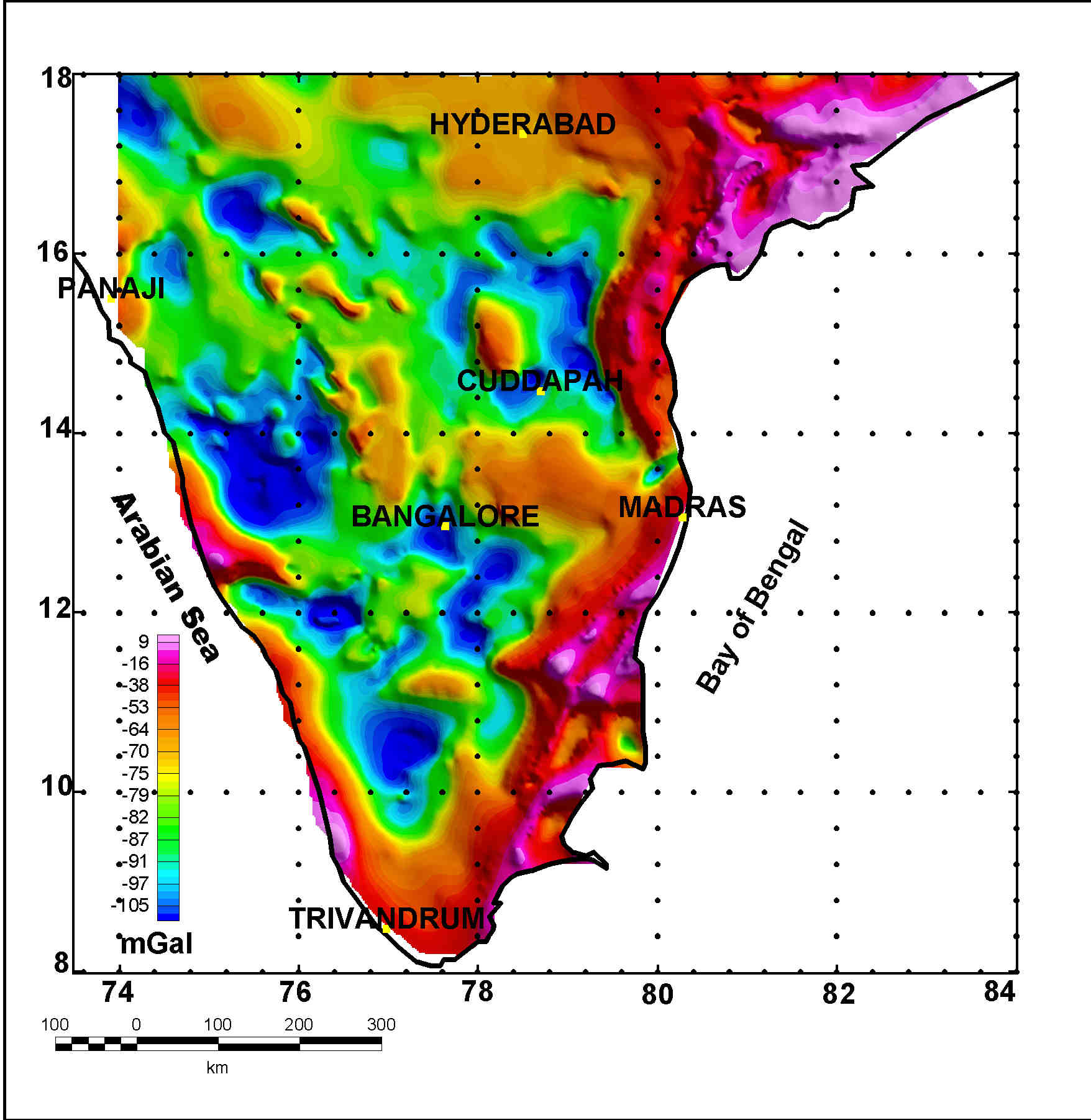
For a comparison of aeromagnetic anomalies with the Bouguer gravity anomalies, we digitized the gravity map (NGRI, 1975) closely along contours and used a grid interval of 2 km to generate the colour image reproduced in Figure 4. The coastal sedimentary basin areas and the Eastern Ghat mobile belts depict gravity high values suggesting high density material in the sub-surface. West of the Chitradurga Boundary fault the gravity map depicts low implying that the Chitradurga Boundary fault represents the divide between the Western and Eastern Dharwar. Signature of the Cuddapah basin is evident in this map.

To derive further information about the sources, their depths and depth structures, the aeromagnetic anomaly map has been analysed using analytic signal, 3D Euler deconvolution and by undertaking a profile analysis of the aeromagnetic data to coincide with the available DSS profile (Reddy et al., 2003).

Analytic Signal

The absolute value of the analytic signal is defined as the square root of the squared sum of the vertical and the two horizontal derivatives of the magnetic field (MacLeod et al., 2000). This signal exhibits maximum over magnetization contrasts, independent of the ambient magnetic field and source magnetization directions. Locations of these maxima thus determine the outlines of magnetic sources. The analytical signal of the total magnetic field reduces the magnetic data to anomalies whose maxima mark the edges of the magnetised bodies. At low latitudes, an extensive source body will have stronger analytical signal at their north and south edges. Figure 5 depicts the analytic signal of the aeromagnetic anomalies over the region.

We find that the analytic signal peaks (sources) within the Dharwar region are of the type that represent intrusives / localised iron ore bodies. At 13∞N parallel, the trends of the maxima align itself along the E-W direction parallel to the orthopyroxene isograd. In fact we can map the orthopyroxene isograd from this map. The zone between Moyar Bhavani-Salem -Attur faults and the Achankovil shear zone is characterized by many maxima representing extensive sources signifying that the host province is magnetic, they are related to the charnokites (higher grade of metamorphism of the host province rocks). Thus the analytic signal can be used to define the change in grades of metamorphism in the subsurface. In fact, the charnockites in the subsurface and in inaccessible regions like forests, etc can be mapped using the analytic signal map. The West Coast fault is clearly visible. Also surprisingly no signatures of the Khondalite belts are evident in this picture though they show clear highs in the aeromagnetic anomaly map; this is because there exists low gradients over the Khondalite belts in the aeromagnetic map.

The analytic signal map shows that within the Dharwars the iron ore deposits of Sandur, Goa, Kudremukh and the intrusives in Cuddapah are distinctly visible. Quite surprisingly the signatures of the Closepet granites show up clearly in this map as a series of intrusives, though it is not quite evident directly in the aeromagnetic anomaly map. The Chitradurga schist belt is not appearing as a single unit but is bisected. Chitradurga schist belt is found terminated towards north by a NE-SW trending linear magnetic source, which has no surface manifestation. This may possibly represents sub-surface dyke system. West of Chitradurga is devoid of magnetic sources expect for the iron ore belts and formations of Bababudan, Kudremukh and Goa. The NNW-SSE trending magnetic sources below Panaji can possibly be related with sub-surface iron ore formation. Thus in the western Dharwar block, iron ore formations is forming a band running almost parallel to the coast line from north of Panjim and kind of joining the iron ore formations of Bababudan and Kudremukh. Major magnetic sources lies to the east of Chitradurga having NW-SE trend. The NW-SE trending Kolar type schist belt is associated with prominent magnetic sources. The Hungund-Kustighi and Raichur-Deodug belt to the north, Veligullu and Ramagiri belt to the southern and central parts respectively show magnetic response (Anand and Rajaram, 202). Towards the Eastern ghat mobile belt, the magnetic sources seen can be associated with the high-grade rocks, mainly charnockites, exposed and in the sub-surface towards the coast and the Nellore greenstone belt. Signatures of the Sileru Shear (10) are clearly evident here.

Euler

3D Euler deconvolution is a technique applied to gridded potential field data (Reid et al., 1990) to help determine the position, depth and nature of any source present. The method is a generalization of EULDPH algorithm that was applied to profile data in Thompson (1982). The method solves Euler’s homogeneity equation for source position, working on a moving window of the grid

(x-x0)dT/dx + (y-y0) dT/dy + (z-z0) dT/dz = N (B-T)

where (x0,y0,z0) is the position of a magnetic source whose total field T is detected at location (x,y,z). The total field has a regional field B; N is the degree of homogeneity and may be interpreted as the structural index (SI) that is a measure of rate of change of the potential field with distance. For example the magnetic field of a point dipole falls off as the inverse cube and could be represented by a structural index of three while a narrow vertical pipe gives rise to an inverse square field fall-off and would be related to a structural index of two. Although these integers represent an ideal relationship between structural index and source type, for real data the source could be represented by a structural index that lies within a range of real numbers. The optimum source location is found by least squares inversion of the data within a chosen window length. Solutions are generally obtained for different SI = 0, 0.5, 1.0, 1.5,2,3 and the solutions with the best clustering of data are selected. The advantages of this method compared to the other classical methods for depth estimation are:

∑ No particular Geological Model is assumed.

∑ Euler’s equation is insensitive to magnetic inclination, declination and remanence

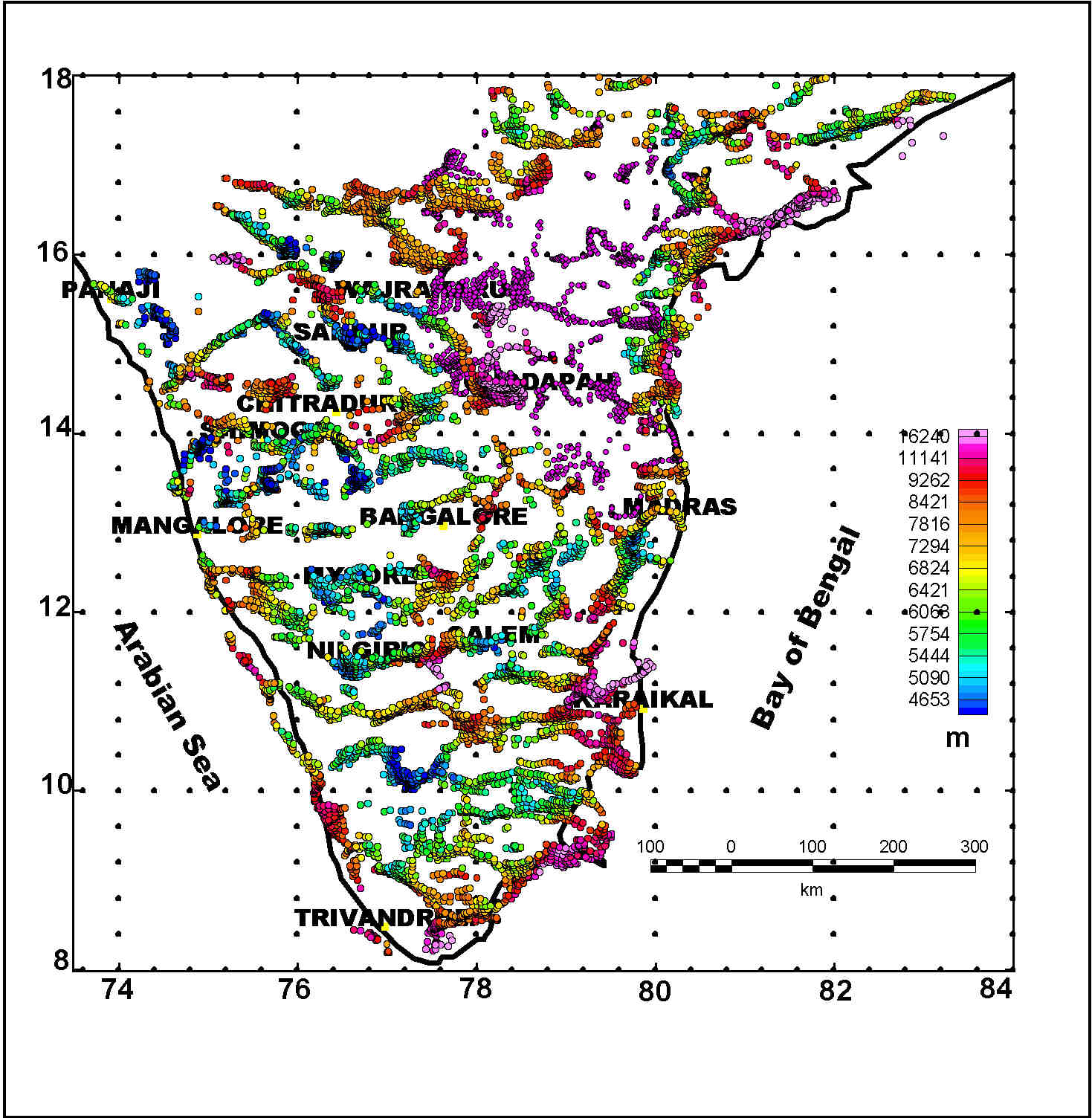
The Euler solutions for the aeromagnetic anomalies give very interesting results. The Euler solutions were generated for different structural indices and using different grid intervals. We found that with smaller grid interval the solutions were noisy. The Euler solution presented here are for grid interval of 5km. The best solutions (tight clustering) were obtained for SI = 2. Figure 6 depicts the Euler solution obtained with the deeper sources represented by warm red colours.

The Euler solutions as seen in Figure 6 would give an idea of the depth estimate of the magnetic sources. It may be noted that the exposed charnockites, due to weathering may have their susceptibility lower than the sub-surface charnockites that would then represent the magnetic sources. The Euler solutions along the Achankovil Shear (26) shows shallower sources on the exposed charnockites and dips southeast to greater depths. The West Coast fault between 10 and 11o N is shallow implying the West Coast fault maybe dissected. The crystalline sedimentary contact fault (6) does show deep sources. Further, the sources along the Cauvery fault (24) are deep, with the fault being terminated by the Bhavani lineament (19). It is interesting to note that the source depths are shallow around the region where the charnockites are exposed and we have deeper sources reflecting the sub-surface charnockites. The Euler solutions could thus be used to study the rate of exhumation within the region.

The sources along the Chitradurg fault appear to be terminated by a NE-SW lineament to the north of Dharma-Tungabadhra lineament (4). The area under study is very large and in order to utilize the Euler solutions appropriately one needs to look at these solutions within small areas. The present study, however, does indicate that one could derive valuable information from Euler solutions. Surprisingly the Euler 3D solutions of the gravity anomaly map over Peninsular India does not depict some of the important shears and contacts brought out by the magnetic solutions eg. Achankovil shear zone. However, the gravity Euler 3D solutions clearly brings out the contact between the sedimentary and the crystallines and the Eastern boundary thrust of the Cuddapah basin. The Chitradurga boundary fault has its signature on the magnetic as well as Bouguer gravity solutions.

Model

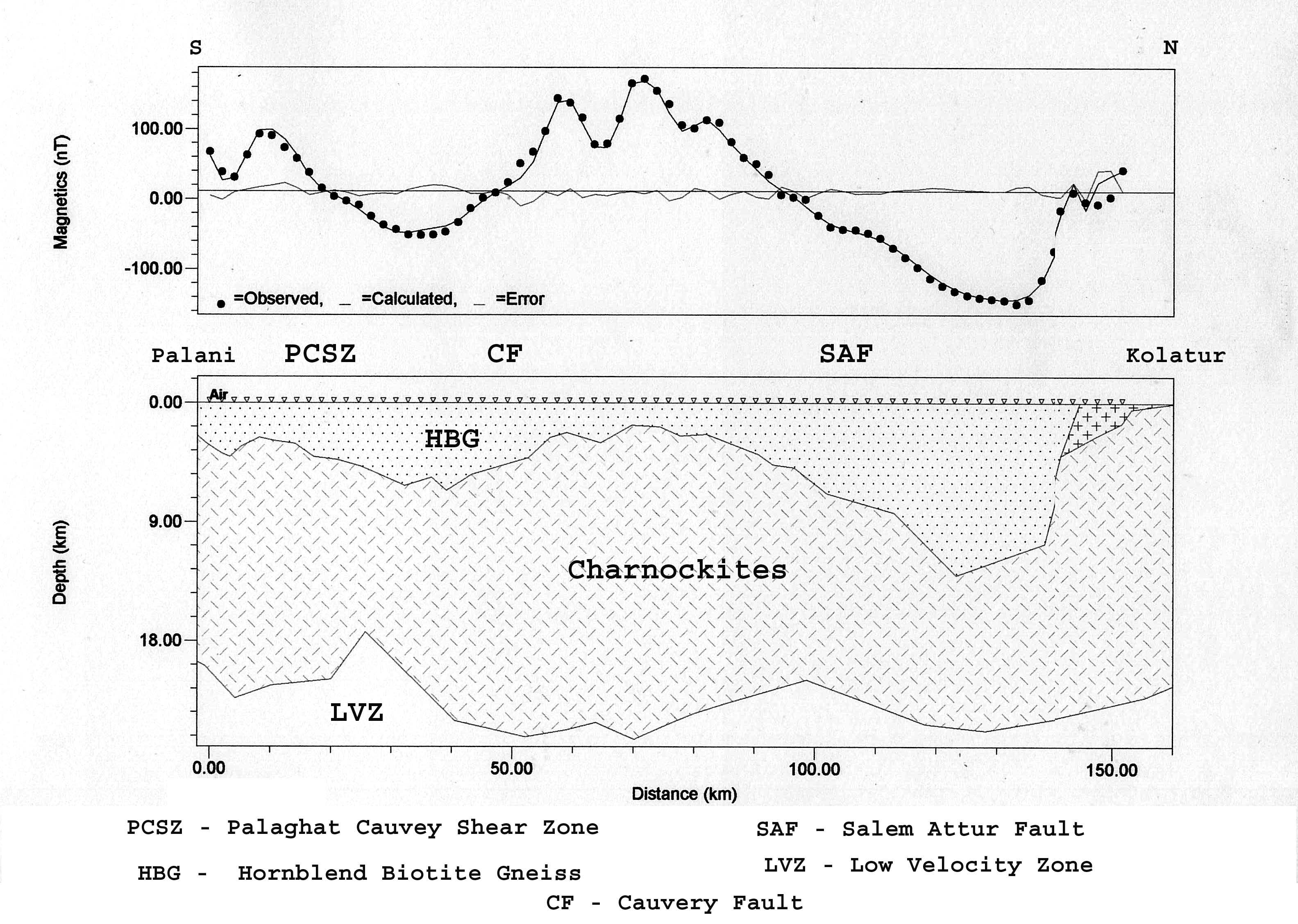
The Department of Science and Technology, Government of India, under its Deep Continental Studies (DCS) Program, identifies challenging and critical areas of research and selects transect corridors for integrated multidisciplinary research to be carried out on a National scale by involving Universities, National Institutions, Survey organizations amongst others. One of the successfully completed multidisciplinary transect is the Kuppam-Palani transect in South India wherein DSS, Magneto telluric, geochemical, gravity, etc studies have been undertaken in this program. Results of the research have been published as a book (Ramakrishnan, 2003). For the forward modeling a profile of the aeromagnetic data is selected along this existing DSS profile (Reddy et al., 2003) from Palani in the south to Kolatur in the north with a total length of 152 km. The location of this profile is superposed on the aeromagnetic anomaly map (Figure 3). The exposed geological formations from Palani to Kolatur along this profile include Hornblend biotite gneiss towards the south and central part and charnockites in and around Kolatur (Reddy et al., 2003). The profile also traverses through the Palaghat-Cauvery Shear Zone, Cauvery Fault and Salem-Attur Fault. The magnetic crust in SGT is thin (Rajaram et al., 2003), with the deeper layers not contributing to the magnetic signatures. The magnetic sources extends to a depth of 22km, below which is a low velocity layer as evidenced in the DSS studies (Reddy et al., 2003). In this model, we therefore constrain the exact depth of charnockites from the DSS profile. From the analysis of aeromagnetic data, it’s analytic signal and filtered map it has been found that charnockites are the main sources of magnetic anomalies in this region. All these information have been incorporated to develop an initial model.

A software program called GM-SYS was used for the modeling. GM-SYS uses a Marqardt inversion algorithm. The forward model incorporates a two-dimensional, flat earth model that is based on geological constraints; the difference between the observed magnetic data and calculated magnetic response to this model (Talwani and Heirtzler, 1964) is minimized by reshaping the model, or by altering the physical properties of the structural units contained within eg., susceptibility. Inversion algorithms within GM-SYS compute an earth model based on the observed field data and a user-specified starting model. The inversion is used to optimize the initial model; therefore, a poorly formed starting model will result in unreasonable solutions. Geopotential models are inherently non-unique, so several model may fit the data equally well. Measured physical properties such as rock susceptibility can constrain the models to geologically reasonable ones. The most reasonable model that fit the data is chosen.

The initial model parameters used are as follows:

The location of the magnetic sources (charnockites) was identified from the analytical signal map. The depth to the bottom of the magnetic sources is taken from the DSS studies along this profile. The initial model is constructed using the available geological information. The susceptibility values for the different rock formation in the area viz. hornblend-biotite gneiss (454µcgs units) and charnockites (2897µcgs units) were incorporated from the laboratory measurements made by Ramachandran (1990).

The magnetic data were modeled starting with the above-discussed parameters and the depth of the layers was interactively modified to reduce the error. For each theoretical model the magnetic response was calculated and compared with the observed. The best-fit model obtained is reproduced in figure 7. The location of the Palaghat-Cauvery Shear Zone (PCSZ), Cauvery Fault (CF) and Salem-Attur Fault (SAF) is shown in the figure . The charnockites with a susceptibility of 2897 µcgs units was used as the basement rock. The modeling of magnetic anomalies shows that the alteration of charnockites into hornblend- biotite- gneiss is more towards the north than south implying that the processes of retrogression in this region is high. From the present model it can be seen that the exhumation of charnockites is more between CF and SAF. Again, towards the south of PCS the exhumation process is high. To check the validity of the model we also made model calculations to reproduce the bouguer gravity values along the same profile; we used the best-fit model obtained from magnetic data as the upper layer with the lower layers taken from the DSS profile for initial model. With minor changes in the depth of the lower layers, we were able to reproduce the gravity anomaly fairly well. This lends credence to the magnetic model. The gravity profile along the DSS has been modeled (Singh et al., 2003) as due to the presence of high-density material (2.80gm/cc) in the upper crust. Our simple model suggests an alternative model where there is no need to involve any intrusives within the country rock.

Conclusion

1. The preparation of an accurate aeromagnetic anomaly map is very crucial to the study of crustal features and the data grid spacing plays a crucial role in the resolution of the anomalies.

2. Three main tectonic features inferred are the Dharwars, Eastern ghat and SGT with the Chitradurga fault dividing the Dharwar into Western and Eastern blocks.

3. The analytical signal can be used to study the change in metamorphic grades and map the charnockites in inaccessible regions and in the subsurface.

4. The Euler solutions can be used to study the extent of exhumation.

5. The aeromagnetic anomalies show much larger variations than the gravity anomalies due to the larger susceptibility variations than density variations of the crustal rocks. In particular this has great relevance to the different metamorphic grades of the crustal rocks.

References

• Anand S.P. and Mita Rajaram, 2002. Aeromagnetic data to probe the Dharwar craton, Current Science 83, 162-167
• Bahuleyan K., 1997. Indian Magnetic Mapping Project – an attempt at aeromagnetic assembly for India in the Global Context; In: Proceedings of the workshop on Airborne Geophysics (ed) Colin V Reeves Association of Exploration Geophysics India. 77-84.
• Balakrishnan, T.S., 1997. Major Tectonic Elements of the Indian Subcontinent and Contiguous Areas: A Geophysical Review; Geol. Soc. of India Memoir 38 103-105
• Geological Survey of India, 1995. Geological map of India, scale 1:5million.
• Geological Survey of India, 2000.Seismo Tectonic Atlas of India and its Environs.
• Geological Survey of India, 2001. Tectonic Map of India, 1:2 million scale and its explanatory brochure (compiled by Sarkar,A.N).
• Geosoft, 1999. Oasis Montage Data Processing and Analysis (DPA) systems for Earth Science applications (ver.4.3), Geosoft Inc.
• Harikumar P., Mita Rajaram and T.S. Balakrishnan, 2000. Aeromagnetic study over Peninsular, India. Proc. Indian Acad. Sci (E&P) 109, 2000, 381-391.
• NGRI/GPH-2, 1975. Bouguer gravity anomaly map of India, 1: 5 million scale.
• MacLeod Ian N., K.Jones and Ting Fan Dai, 2000. 3-D Analytic Signal in the Interpretation of Total Magnetic Field Data at Low Magnetic Latitudes (Research papers Geosoft Inc.)
• Mahadevan, T.M., 2003. Geological evolution of the South Indian shield – Constraints on modelling, Mem. Geol. Soc. India, Ed. M.Ramakrishna, 50, pp 25-46.
• Prabhakar, K.N. and P.L.Zutshi, 1993. Evolution of southern part of Indian East Coast Basin, J. Geol. Soc.India, 41, 215-230.
• Project Vasundhara, 1994. Special Publication AMSE Wing Geological Survey of India Bangalore.
• Rajaram Mita and S.P. Anand, 2003. Central Indian tectonics revisited using Aeromagnetic data, Earth Planets Space, 55, e1-e4.
• Rajaram Mita, S.P.Anand and V.C.Erram, 2000. Magnetic studies over Krishna-Godavari basin in Eastern Continental margin of India, Gondwana Research, 3, 385-393.
• Rajaram Mita, P. Harikumar and T.S. Balakrishnan, 2001. Comparison of aero and marine magnetic anomalies over peninsular India, J. Geophysics, 22, 11-16.
• Rajaram Mita, P. Harikumar and T.S. Balakrishnan, 2003. Thin Magnetic Crust in the Southern Granulite Terrain, in: Tectonics of Southern Granulite Terrain, Kuppam-Palani Geotransect, M. Ramakrisnan (ed.), Mem. Geol. Soc. India, 50, 163-175
• Ramachandran,C., 1990. Metamorphism and Magnetic susceptibilities in South Indian Granulite Terrain, Jour. Geol. Soc. Ind., v.35, 395-403.
• Ramakrishnan,M., 2003. Tectonics of Southern Granulite Terrain, Kuppam-Palani Geotransect, (ed.), Mem. Geol. Soc. India, 50.
• Reddy, A.G.B., M.P.Mathew, Baldau Singh and P.S. Naidu, 1988. Aeromagnetic evidence of crustal structure in the granulite terrain of Tamil Nadu- Kerala; Journal of Geol. Soc. of India 32 368-381.
• Reddy, P.R., B.Rajendra Prasad, V.Vijya Rao, Kalachand Sain, P.Prasad Rao, Prakesh Khare and M.S.Reddy, 2003. Deep seismic reflection and refraction/wide-angle reflection studies along Kuppam-Palani transcet , in: Tectonics of Southern Granulite Terrain, Kuppam-Palani Geotransect, M. Ramakrisnan (ed.), Mem. Geol. Soc. India , 50, 79-106.
• Reid,A.B., J.M. Allsop, H. Granser, A.J. Miliett, and W.I Somerton, 1990. Magnetic
• interpretations in three dimensions using Euler deconvolution, Geophysics., 55, 80-91.
• Roest,R.W., J.Verhoef, and M.Pilkington, 1992. Magnetic interpretation using the 3-D analytic signal Geophysics, 57, 116-125.
• Sarkar A.N., 2001. Explanatory brochure on the Tectonic map of India, Geological Survey of India.
• Singh,A.P., D.C.Mishra, V.Vijya Kumar, and M.B.S. Vyaghreswara Rao, 2003. Gravity and Magnetic signatures and crustal architecture along Kuppam-Palani geo-transect, South India, in: Tectonics of Southern Granulite Terrain, Kuppam-Palani Geotransect, M. Ramakrisnan (ed.), Mem. Geol. Soc. India, 50, 2003, 125-138.
• Subrahmanyam, C. and R.K.Vemra, 1982. Gravity interpretation of the Dharwar Greenstone-Gneiss-Granite terrain in the south Indian shield and its geological implications, Tectonophysics.
• Swami Nath, J., M.Ramakrishnan and M.N.Viswanatha, 1976. Dharwar Stratigraphic model and Karnataka craton evolution. Rec. Geol. Surv. India, 107, 149-175.
• Talwani, M., and J.R.Heirtzler, 1964. Computation of magnetic anomalies caused by two-dimensional bodies of arbitrary shape, in Parks, G. A., Ed., Computers in the
• mineral industries, Part 1: Stanford Univ. Publ., Geological Sciences, 9, 464-480.
• Thompson, D.T., 1982 EULDPH – A new technique for making computer assisted depth estimates from magnetic data, Geophysics, 47, 31-37.

Figures

Figure 1

Detailed geology and tectonic map of Peninsular India (redrawn from GSI, 1995, 2000, Project Vasundhara, 1994). KGB – Krishna-Godavari Basin, CB – Cauvery Basin, CDB – Cuddapah Basin 1. Benni Hall Lineament, 2. Krishna River Fault, 3. Chitradurga Boundary Shear, 4. Dharma – Thungabhadra Lineameant, 5. Kumudvati – Narihalla Lineament, 6. Crystalline-sedimaentary contact fault (A), 7. Kurnool – Kolhapur Lineament, 8. Dindi Fault, 9. Nallamali Shear, 10. Sileru Shear, 11. Eastern Boundry Thrust, 12. Bhadra Lineament, 13. Hemavati Lineament (A), 14. Vedavati Lineament, 15. Hunsur Lineament, 16. Arkavati Fault, 17. Bhavali Lineament , 18. Moyar Fault, 19. Bhavani Lineament, 20. Mettur East Fault (A), 21. Salem-Attur Fault (Godumalai Shear Zone) (A), 22. Palar River Fault (A), 23. Attur Fault, 24. Cauvery Fault, 25. Vaigai River Fault, 26. Achankovil shear zone, 27. Tenmalai (Punalur) Fault. The seismically active faults are denoted by (A).

Figure 2

Epoch and altitude of aeromagnetic survey undertaken. Different flight altitudes are indicated in different colours: light blue – 5000’, dark blue – 7000’, yellow – 9500’, purple – 500’.

Figure 3

Aeromagnetic anomaly map of South India. Red colour depicts high and blue depicts lows. The location of the aeromagnetic profile, chosen along the existing DSS profile and discussed in the text, is overlain.

Figure 4

Bouguer Gravity anomaly map of the region redrawn from NGRI (1975).

Figure 5

Analytic signal map of the aeromagnetic anomaly. Red colour represents magnetic sources (highs).

Figure 6

Magnetic source depth and location using Euler deconvolution. (window length=10, structural index = 2, with data grid of 5 km).

Figure 7

Crustal Model based on surface geology (Reddy et al., 2003) to reproduce the observed aeromagnetic anomaly along the DSS profile: Palani-Kolattur. The susceptibility values are based on published literature (Ramachandran, 1990). The source locations are taken from the analytical signal map and the initial depths are based on DSS (Reddy et al., 2Figure 7. Crustal Model based on surface geology (Reddy et al., 2003) to reproduce the observed aeromagnetic anomaly along the DSS profile: Palani-Kolattur. The susceptibility values are based on published literature (Ramachandran, 1990). The source locations are taken from the analytical signal map and the initial depths are based on DSS (Reddy et al., 2003).