Kayal, J.R. 2003. Seismic Tomography Structures Of Source Areas Of The Two Recent Devastating Earthquakes In Peninsular India.
Journal of the Virtual Explorer 12, 66-71.
Seismic Tomography Structures Of Source Areas Of The Two Recent Devastating Earthquakes In Peninsular India.
Abstract
Seismic tomography structures of source areas of the 1993 Killari earthquake (mb 6.3) in central India and the 2001 Bhuj earthquake (MW 7.5) in western India are studied. The tomography images revealed lateral heterogeneities and depth variation in velocity; the main shocks occurred in the high velocity zones at the fault ends. The aftershock locations are improved by the tomography method
Introduction
‘Tomo’ is from a Greek word which means “slice”. In tomography, we examine a series of two-dimensional slices from a three dimensional object, and use the informtions to infer the internal structure of the three dimensional object.
Medical tomograph and seismic tomography share some similarities, but they also have important differences. In medical tomography, we measure the intensity of received x-rays, which is a function of the absorption coefficient of the travel path through human body. In seimic tomography, we measure a travel time which is a function of the slowness (inverse of velocity) along the ray path through the Earth. In medical tomography, the travel path is a straight line. In seismology, the ray path is almost never a straight line.Also, in medical tomography, the source and detector locations are known exactly at all times. In seismic tomography, the earthquake source locations are unknowns which must be solved for, while inverting for the seismic or velocity structure. Thus a simultaneous inversion technique is used in seismic tomography to reveal the velocity structure, at the same time source parameters of the seismic events.
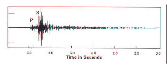
In this paper we shall be discussing tomography structures of the source areas of the two recent devastating intraplate earthquakes in peninsular India; the 1993 Killari earthquake, body wave magnitude mb 6.3, in central India, and the 2001 Bhuj earthquake, moment magnitude MW 7.5, in western India (Figure 1). These two earthquakes generated large number of aftershocks. Several thousands of P and S arrivals were available for these two aftershock sequences. An example of P and S phases of seismic waves generated by an earthquake is exemplified in figure 2. These seismic arrival times are used for earthquake location as well as for tomography study to reveal the seismic/geologic structures in the crust. The results shed new light in understanding the earthquake source areas, geologic/velocity structures at depths.
It may be mentioned that the 1997 Jabalpur earthquake (mb 6.0) in the Narmada-Son Lineament Zone in central India (Figure 1) did not produce enough aftershocks for tomography study.
Seismic Tomography Method
To parameterize the velocity structure, we superimpose a threedimensional grid on the region of the crust containing the earthquake sources and the seismic stations. Each of the cells within the grid system is assumed to have constant velocity, but the velocity can vary from cell to cell. In practice, the dimensions of each block can be different. For example, around a fault we probably want to have a finer grid than at greater distance from the fault. For better resolution, large number of ray paths should pass through each grid. Thus a large data base with high precision P and S arrivals is required for the inversion.
The simultaneous inversion problem can be posed in the following manner. There is an array of (m) stations indexed k = 1,2, ...., m. The array is used to record (n) earthquakes indexed j = 1,2, ...., n. The hypocentre parameters for the jth earthquake are (tjo, xjo, yjo, zjo). There are n earthquakes, so the complete set of hypocentre parameters is (t1o, x1o,y1o, z1o t2o, x2o, y2o, z2o, ---, tno, xno, yno, zno). There are a total of 4n unknown parameters in this vector. This is a generalisation of the earthquake location problem. In the earthquake location problem, we are given a set of m stations with m corresponding arrival times, and we want to find the best origin time and hypocentre location, assuming a velocity model. We make a starting guess for the desired parameters, and through an iterative procedure, we improve the guess until it meets some stopping criterion. In simultaneous inversion, we do this but we also solve for the velocity model at the same time. Thus the earthquakes are located with better precision.
1993 Killari Earthquake
The Killari earthquake (mb 6.3) of September 30, 1993, in the Latur district of Maharashtra State, Central India, killed about 7,500 people (GSI, 1996). It occurred in the middle of the continental shield in a region of low seismic activity (Figure 1). The local geology in the area is obscured by the late Cretaceous-Eocene basalt flows, referred to as Deccan traps. This makes it difficult to recognise the geological surface faults that could be associated with the Killari earthquake. The epicentre was reported at 18.090N and 76.620E (IMD report), and the focal depth at 7 + 1 km was precisely estimated by wave form inversion (Chen and Kao, 1995).
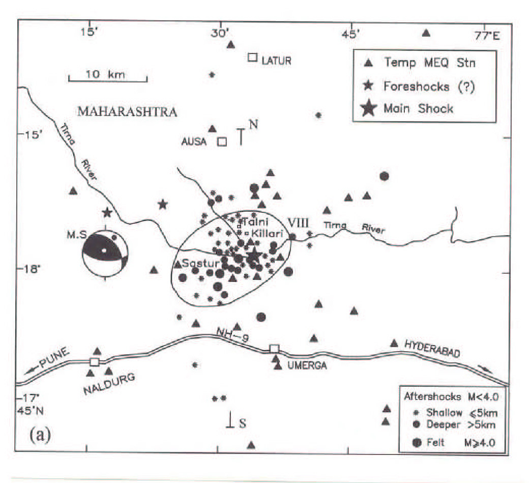
The aftershock investigation was carried out by making a temporary microearthquake (MEQ) network by the GSI (1996). 140 aftershocks were well located by the GSI network; the epicentres are shown in Figure 3a. Almost all the epicentres are located within the meizoseismal area, in the hight intensity (VIII) zone. Most of the aftershocks (77%) are of shallow origin, depth 0-<6 km, and rest of the events occurred at a depth range 6-15 km. A detailed discussion on the seismotectonics of the main shock and aftershocks is given by Kayal (2000).
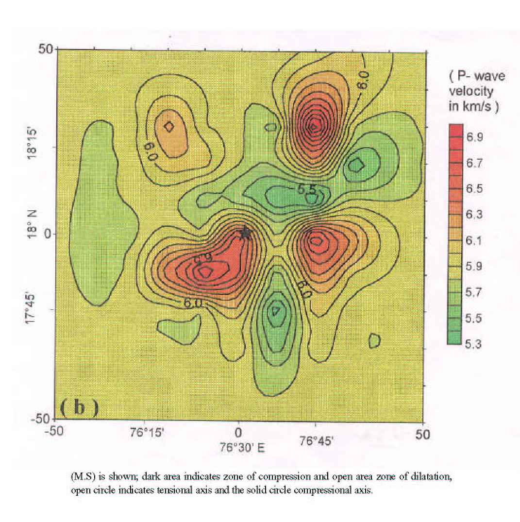
About 2700 seismic arrivals, 1500 P and 1200 S, were available from the temporary networks of GSI and NGRI for the tomography study (Kayal and Mukhopadhyay, 2002). Local Earthquake Tomography method of Thurber (1983), modified by Eberhart-Phillips (1993), is used in this study. In this method the location errors (rms, epicentre, depth) are improved, and the lateral heterogeneity of the velocity structure is revealed. The tomography structure at a depth of 6 km, at the main shock source area, is illustrated in Figure 3b. An E-W trending low velocity zone (LVZ) is prominent with another N-S trending LVZ to its south. The main shock occurred at the contact between the E-W trending LVZ and a high velocity zone (HVZ) to its southwest (Figure 3b). The E-W trending LVZ possibly indicates the seismogenic fault at this depth, and the main shock occurred at the fault end.
2001 Bhuj Earthquake
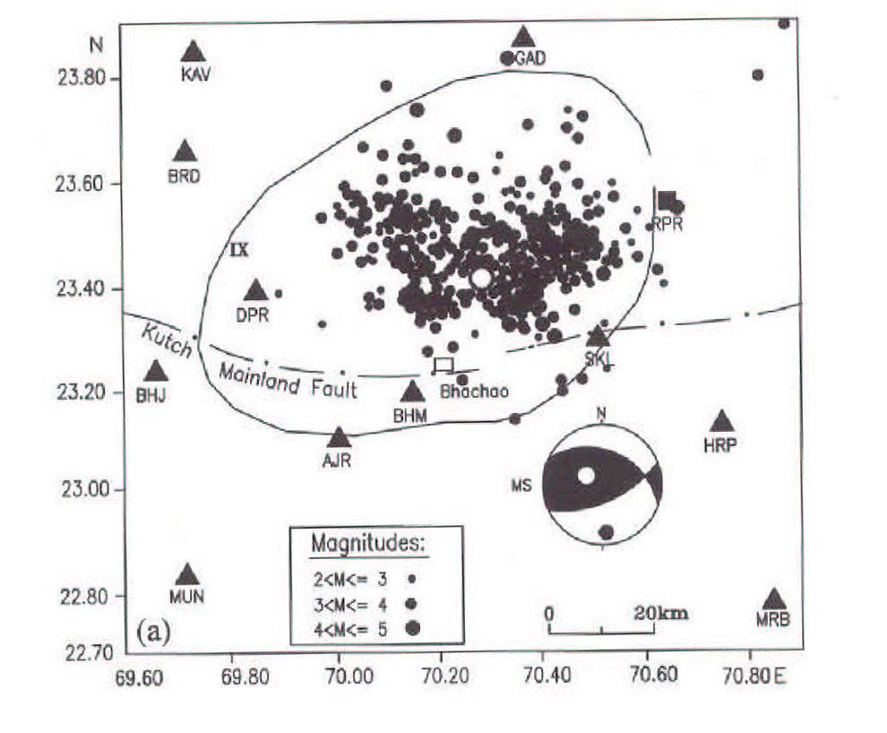
The devastating Bhuj earthquake (MW 7.5) of January 26, 2001 in the Gujarat state, in the northwestern part of peninsular India, rocked the whole country, and killed about 15,000 people. The epicentre of the earthquake is reported at 23.400N and 70.280E, and the well estimated focal depth at 25 km (IMD Report). A total of about 3000 aftershocks (M>2.0) were recorded till mid April, 2001 (Kayal et al., 2002a). The epicentre map shows an aftershock cluster area, about 60 km x 30 km, between 70.0-
70.60E and 23.3-23.60N; almost all the aftershocks occurred within the high
intensity (IX) zone (Figure 4a). The source area of the main shock and most of the aftershocks is at a depth range 20-35 km. A detailed report on the seismotectonics of the Bhuj earthquake sequence is given by Kayal et al., (2002a).
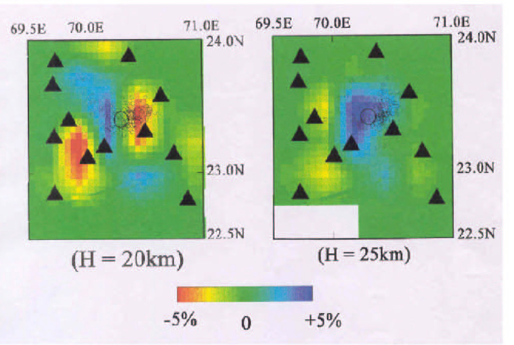
Out of 3000 aftershocks, 331 events were selected for the tomography study (Figure 4a). A total of 3813 seismic phases, 1948 P and 1865 S arrivals, are used. A 3-D grid was set up in the study area with grid spacing 20 km in horizontal direction and 5 km in depth. In this study we have used the tomography software of Zhao et al. (1992) at the Geodynamic Research Centre, Japan ; the detailed results are given by Kayal et al. (2002b). The tomography images at the main shock source area, depth 20-25 km, reveal interesting structures. It depicts two LVZs, and in between a HVZ at a depth of 20 km (Figure 4b). The main shock and the aftershocks are bounded by the HVZ and by the LVZ to its east. The tomography images at a depth of 25 km show no LVZ; the HVZ is prominent in the source area (Figure 4b). It implies that the tectonic stress accumulated within the HVZ, and the main shock nucleated at the fault end within the HVZ.
Conclusion
The Seismic Tomography is a state-of-the-art technique in earthquake location and velocity structure study. The tomography results of the 1993 Killari and the 2001 Bhuj earthquake source areas show that the high velocity zones (HVZ) at the fault ends are the source zones for the stress accumulation. The main shocks nucleated at the fault ends, within the HVZ or at the contact zone.
References
- Chandra, 1977. Earthquake of Peninsular India - A Seismotectonic study, Bull. Seism. Soc. Am., 67 : 1387-1413.
- Chen, W.P. and Kao, H., 1995. Seismotectonics of Asia : Some recent progress, In : The Tectonic Evolution of Asia, ed : A. Yin and M. Harrison, Cambridge Univ. Press, New York, 280p.
- Chung, Wai-Ying and Gao, H., 1995. Source parameters of the Anjar earthquake of July 21, 1956, India and its seismotectonic implications for the Kutch rift basin, Tectonophysics, 242 : 281-292.
- Eberhart-Phillips, D., 1993. Local earthquake tomography : Earthquake source region : In Seismic Tomography : Theory and Practice, ed. H.M. Iyer and K. Hirahara, Chapman and Hall, London, P. 613-643.
- GSI, 1996. Killari Earthquake, 30 September, 1993, Geol. Surv. India Sp. Pub. 37, ed. P.L. Narula, S.K. Shome and B.S.R. Murthy, 282p.
- Kayal, J.R. 2000. Seismotectonic study of the two recent SCR earthquakes in Central India, J. Geol. Soc. India, 55 : 123-138.
- Kayal, J.R. and Mukhopadhyay, S., 2002. Seismic tomography structure of the 1993 Killari earthquake source area, Bull. Seism. Soc. Am. (in press).
- Kayal, J.R., De, Reena, Sagina Ram, Srirama, B.V. and Gaonkar, S.G., 2002a. Aftershocks of the January 26, 2001 Bhuj earthquake and its seismotectonic implications, J. Geol. Soc. India, 59: 395-417.
- Kayal, J.R., Zhao, D., Mishra, O.P., De, Reena and Singh, O.P., 2002b. The 2001 Bhuj earthquake : Tomography evidence for fluids at hypocentre and its implications for rupture nucleation, Geophys. Res. Lett. (Submitted).
- Ravi Shanker and Pande, P., 2001. Geoseismological studies of Kutch (Bhuj) earthquake of 26, January, 2001, J. Geol. Soc. India, 58: 203-208.
- Thurber, C.H., 1983. Earthquake location and three dimensional crustal structure in the
- Coyote Lake area, central California, J. Geophys. Res. 88, B10 : 8226-8236.
- Zhao, D., Hasegawa, A. and Horiuchi, S., 1992. Tomographic imaging of P and S wave
- velocity structure beneath northeast Japan, J. Geophys. Res., 97 : 19,909-19,928.
Figures
- Figure 1
- Map showing epicentres of the major tectonic features and the significant earthquakes (M ‡ 5.0 ) in penisular India; the recent damaging earthquakes are shown by star symbols. Preferred fault-plane solutions are shown (1-6 : after Chandra, 1977; 7 : Chung and Gao, 1975; 8-10 : USGS); the dark area indicates the zone of compression, and the blank area zone of dilatation, the fault movement is shown by arrows. NSL : Narmada Son Lineament, NNF : Narmada North Fault, NSF : Narmada South Fault, TL : Tapti Lineament, KMF : Kutch Mainland Fault. Inset : Indian plate movement from the Carls Berg Ridge (CBR), HA : Himalayan Arc, BA : Burmese Arc.
- Figure 2
- A digital seismogram showing P and S arrivals of an aftershock, magnitude 2.1, in Bhuj area.
- Figure 3a, 3b
- (a) Map showing epicentres of the Killari earthquake of September 30, 1993 and its aftershocks. The solid circles indicate deeper (6-15 km) aftershocks and the small stars shallower (0 -<6 km) aftershocks. The high intensity zone, isoseismal VIII, is shown by curved line (GSI, 1996). The fault-plane solution (lower hemisphere) of the main shock (b) Seismic tomography images at a depth of 6 km, the star indicates the main shock. P-wave velocity contours are shown with colour code.
- Figure 4a, 4b
- (a) Epicentre map of the Bhuj earthquake of January 26, 2001 and its aftershocks. The main shock is shown by the bigger open circle, and the aftershocks by solid circles. The fault plane solution of the main shock is shown. The isoseismal IX is shown after Ravi Shanker and Pandey ( 2001). (b) Seismic tomography images at depths 20 km and (c) at 25 km. P-wave velocity perturbation (in %) is mapped. (Note : Change in colour code). The main shock and the aftershocks at these depths are shown.