Discussion
VS structures and geophysical constraints
Since the non-linear inversion and its smoothing optimization guarantee only the mathematical validity of the selected structural models, independent geophysical information (e.g. Moho depth, seismicity and heat flow) are used as additional constraints whenever necessary. The structural models selected by LSO are appraised with respect to independent information available in the literature concerning the Moho boundary depth (Dezes and Ziegler, 2001; Tesauro et al., 2008; Grad and Tiira, 2008). More than half of the cells in the study area have the Moho depth in accordance with the average value reported by Dezes and Ziegler (2001). Moreover, comparing the Moho depth resulting from our model, taken with its uncertainties, to the minimum and maximum depth reported by Tesauro et al. (2008) and Grad and Tiira (2008), for each cell, the agreement rises to about 90%.
Some of the cells that have Moho depth in disagreement with the above cited literature can be considered as influenced by border effects, i.e. the cells are at the border of the study area and could not be constrained well by the optimization algorithms. In these cells we choose among the cellular set of solutions the one that has crustal thickness in agreement with the values in the literature, if such solution exists. This is the case for cells e7, c10, b10 and D4. The selected models correlate well with the observed seismicity-depth distribution. Cells B-2 and g-2 are on the border of the study area and present a crust thinner than the values reported in the literature, but among the set of solutions for both cells there is no model that has values for the Moho depth closer to the published ones. Anyway, we consider the modelled crustal depth for cell B-2 to be realistic, since the obtained VS model is derived from surface wave data with good coverage, especially in the Sardinia region and we do not know any other more detailed study of the Sardinian crustal structure.
The main differences are observed in cells where a steep Moho gradient is present (i.e. collisional or subduction zones and oceanic-continental boundaries). The crustal structure of these cells is discussed below.
In cell B8 (Ionian Sea), a crust 27 km thick is modelled that is thinner than that reported in the literature. Among the solutions for the cells there is no model with thicker crust, therefore we consider our result more reliable.
In cells A-2, A-1 and A5 the Moho depth is shallower than the values reported in the literature, but the obtained values are well correlated with a geological section crossing these cells (discussed in detail in Panza et al., 2007b).
In cell d4 a crust (25-27 km) thinner than that reported in the above cited literature (30-42 km depth) is modeled, but a recent study of Šumanovac et al. (2009) indicates a crust less than 30 km thick in the Quarnaro Gulf. Moreover, the cellular seismicity deeper than 20 km is almost absent. The underlying soft mantle layer (VS ~ 4.10 km/s) has a thickness of about 34 km, reaching 60 km of depth. The observed heat flow in this cell is low, about 40 mW/m2.
The selected model for cell a-1 has a thin, about 16 km, crust that overlies a soft mantle layer with VS of about 4.20 km/s that reaches the depth of 28 km. The cellular seismicity is weak and the heat flow values do not exceed 70 mW/m2.
In cell a1 the Moho is observed at about 6 km of depth. The crust overlies a LID layer with VS of 4.70-4.80 km/s that reaches the depth of about 10 km. The following 10 km thick soft mantle lid, with VS of 3.65-3.85 km/s, is the most probable source of the observed high heat flow (150 mW/m2). The structure of the cells is in accordance with the petrological interpretation that is discussed in detail by Panza et al. (2007a).
In cell A3 the crust reaches the depth of about 6 km and overlies a layer with VS 4.20-4.60 km/s extended down to 11 km of depth. The underlying layers have VS about 3.50 km/s and 4.00 km/s, respectively, and thickness of about 10 km and 40 km, therefore can be interpreted as soft mantle, in fair accordance with high heat flow (about 150 mW/m2). The velocity structure of this cell is discussed in detail by Panza et al. (2007a) considering the Moho depth at 6 km. Alternatively we could interpret the 5 km thick layer with VS between 4.20 and 4.60 km/s as an Ultra High Pressure (UHP) metamorphosed crust with high percentage of coesite (VS about 4.60 km/s and a density of about 2.9 g/cm3, according to Anderson 2007). In this way, a Moho depth of about 11 km will be in agreement with Moho depth reported in the literature and seismicity-depth distribution. This new interpretation of the velocity structure is not in contradiction with interpretation given in Panza et al. (2007a).
In cell A7 the layer with VS of 4.10 km/s at depths between 20 and 40 km is interpreted as crust with VS range of 4.00 - 4.10 km/s. The thickness of the crust is in the range 35 - 45 km and it is slightly thicker than the maximum values found in the above cited literature (30 – 36 km). However, our interpretation fits well the low heat flow (less than 40 mW/m2) that is observed in the area. Weak seismicity is observed in the cell down to a depth of about 35 km. Similarly in cell c6, the layer with VS about 4.20 km/s, located between 26 and 36 km of depth, is considered to be crustal with VS range from 4.05 to 4.20 km/s. The resulting crustal thickness (about 36 km) is in accordance with the above cited literature values (ranging from 32 to 43 km). The values of the heat flow in the cell are less than 35 mW/m2 (Hurting et al., 1991), correlating well with our interpretation.
In cell a5, the 43 km thick crust is slightly thicker than that reported in the literature (ranging from 29 to 38 km). However, the crustal structure of our model correlates well with observed seismicity, that stops at a depth of about 40 km, and low heat flow (less that 60 mW/m2). Similarly the obtained 49 km thick crust in cell c4 correlates well with significant seismic energy release (down to about 48 km of depth) and low heat flow (less than 45 mW/m2) observed in the cell.
The cell a6 (offshore Apulia) presents a thinner crust (about 20 km) than the published values (ranging from 27 to 38 km). The following mantle layer with VS of 4.05-4.35 right below the Moho is extended to 46 km of depth. The observed seismicity in this layer is weak and heat flow is less than 65 mW/m2.
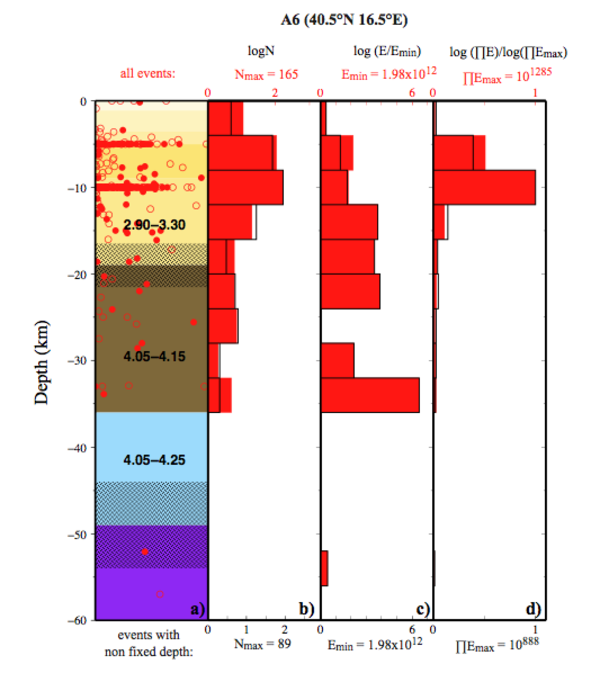
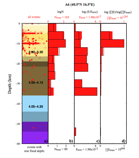
In cell a2, under the Albani hills and the Tyrrhenian offshore, with heat flow reaching 150 mW/m2, the definition of Moho is difficult using VS alone. The Moho is located at 25 km of depth splitting the 29 km thick layer with VS range of 3.90-3.95 km/s into two parts: 19 km thick crustal layer and 10 km thick mantle layer, according to the seismicity-depth distribution (discussed in detail in Panza et al., 2007a; Panza and Raykova, 2008). Similarly in cell e4, at about 23 km of depth, the 30 km thick layer with VS about 4.00 km/s is split in two layers: a 17 km thick crustal layer lying on a 13 km thick soft mantle layer, according to the seismicity distribution that is concentrated in the uppermost 40 km (Panza et al., 2007a). The Moho depth defined in this way for the cells a2 and e4 is in fair agreement with published data. We proceeded similarly for cell A6 (Fig. 10). The values for the crustal thickness range from 32 to 39 km and the heat flow ranges from 30 to 90 mW/m2. In the obtained VS model an upper crustal layer with VS of about 3.10 km/s reaches the depth of 19 km. The following 30 km thick layer has VS from 4.05 to 4.25 km/s. Below this layer a high velocity lid (VS 4.65-4.80 km/s) reaches the top of the asthenosphere at about 80 km of depth. The depth distribution of the observed seismicity is analyzed and the computed histograms are shown in Fig.10. The obtained VS model down to the depth of 60 km is presented in Fig. 10a using the same VS color coding as in Figs. 3-9. The location of the earthquakes with magnitude specified by the ISC catalogue are noted by red dots, while the events without magnitude indication are noted by red circles. The seismicity-depth distribution is presented in several histograms: logN-h distribution (Fig. 10b), logE-h distribution (Fig. 10c), and log∏E-h distribution (Fig. 10d). All three kinds of seismicity-depth distributions are calculated for two selections of events: all events from the ISC catalogue (red histograms, related red-color annotations and text on the top of the Figs 10b, c, and d) and events with depth not fixed a priori in the hypocenter computing (black-line histograms, related black-color annotations and text on the bottom of the Figs 10b, c, and d). The Nmaxin Fig 10b gives the maximal number of the earthquakes in the 4 km thick depth intervals. The Emin in Fig. 10c means minimal sum of energy in the depth intervals, that is greater than 0 and that is used as the normalization factor in log∏E-h calculation. The ∏Emaxin Fig. 10d denotes the maximum of the energy product in the depth intervals, that is greater than 0 and that is used as the normalization factor in logE-h calculation. Analyzing the presented seismicity-depth distributions the clear stop of the seismicity at about 36 km is observed and thus we locate the Moho at this depth. Therefore, the lower crust (17 km thick) with a VS range of 4.05-4.15 km/s lies on a 13 km thick soft mantle layer with a VS range of 4.05-4.25 km/s. The presence of this shallow, thin, and soft mantle layer can be related to the elevated local heat flow data (up to 90 mW/m2).
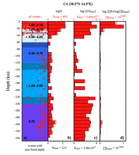
The VS models of the cells where the intensive deep mantle seismicity is observed are correlated with computed seismicity-depth distribution. In cell C4 (Aeolian Islands) the seismicity is observed down to about 340 km and the heat flow is in the range of 75 – 250 mW/m2. The very intensive and energetic seismic-depth distributions in the uppermost 20 km of the structure (Fig. 11a, the symbols that are used are the same as in Fig. 10) indicate the Moho depth of about 20 km. A hot mantle layer follows, with VS about 3.65-4.20 km/s down to 60 km of depth. The seismicity decreases drastically below 20 km of depth and almost stops at a depth of about 50 km. The deep seismicity starts to be notable below 90 km of depth down to about 200 km of depth. The VS at these depths decreased slightly from 4.55 km/s to about 4.40 km/s. The seismic energy release deeper than 220 km increased drastically and this peak correlates very well with the top of the high velocity layer (VS about 4.75 km/s). The observed intense seismicity below a depth of 220 km has almost constant energy release down to a depth of 350 km.
Figure 10. Cell A6: model and seismicity.
The cellular VS structure of cell A6 and distributions of seismicity. The model is plotted on the leftmost graph (a). The VS ranges of variability in km/s are printed on each layer and the hatched rectangles outline the ranges of variability of the layer’s thickness. The values of VS in the uppermost crustal layers are omitted for the sake of clarity. The hypocentres with depth and magnitude type specified in the ISC catalogue are denoted by dots. The hypocentres without magnitude values in the ISC catalogue are denoted by circles. (b) logN-h, distribution of the number of earthquakes with respect to depth obtained by grouping hypocentres in 4-km intervals. (c) logE–h, distribution of the normalized logarithm of seismic energy for 4-km-thick depth intervals. (d) log∏E-h, distribution of the normalized logarithm of product of seismic energy for 4-km-thick depth intervals. The filled red bars histograms represent the computation that used all earthquakes from the revised ISC (2007) catalogue for period 1904–June 2005. The black line histograms represent the computation that used earthquakes which hypocentre’s depth is not fixed a priori in the ISC catalogue. The normalizing values of energy’s logarithm logEmin and product of energy’s logarithm log∏Emaxare given on the horizontal axes of the relevant graphs.
Figure 11. Cell C4: model and seismicity.

The cellular VS structure in cell C4 and related seismicity distribution, obtained grouping hypocentres in 10-km intervals: (a) VS cellular model; (b) logN-h; (c) logE–h; (e) log∏E-h. The symbols used are the same as in Fig. 10.
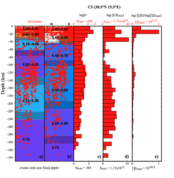
Similarly, very intensive deep seismicity is observed in cell C5 (Fig. 12) (area of Stromboli, Messina Strait and Southern Calabria) down to the depth of about 400 km. The unconstrained VS model selected by LSO is not consistent with the observed seismicity and independent data about the presence of a subducting slab (Panza et al. 2007a). Among the set of solutions for this cell only those consistent with the seismicity are considered and LSO is performed again keeping the solutions in the neighbouring cells fixed. The selected model is further analyzed considering the seismicity in the northern and southern half of the cell separately (Panza et al. 2007a, Panza and Raykova, 2008). The comparison between the unconstrained solution and selected representative cellular model and their correlation with the seismicity distributions is shown in Fig. 12. The unconstrained solution (Fig. 12a) is not consistent with the observed seismicity and known structural features in the region, while the constrained solution shown in Fig. 12b correlates very well with the seismicity-depth distributions (logN-d shown in Fig. 12c; logE-h shown in Fig 12d, log∏E-h shown in Fig 12e; the symbols used are the same as in Fig. 10). It is difficult to define the nature of the crust in the selected VS model, since a layer with VS in the range 3.8–4.0 km/s reaching a depth of about 44 km overlies high velocity mantle material. The analysis of the seismic energy distribution (details given in Panza et al., 2007a; Panza and Raykova, 2008) leads to two distinct interpretations for this two-faced (Janus) crust/mantle layer. Considering only the hypocentres at sea (northern half of the cell), this layer is totally aseismic and therefore it is assigned to the mantle, and the crust in this half of the cell has an average thickness of 17 km. On the other hand, considering only the hypocenters in the continental southern half of the cell, the “Janus” layer is intensively seismic and therefore it is assigned to the brittle continental crust which turns out to be 44 km thick.
Figure 12. Cell C5: model and seismicity.
The cellular VS structure in cell C5 and related seismicity distribution obtained grouping hypocentres in 10-km intervals: (a) the unconstrained model selected by LSO; (b) the representative cellular model; (c) logN-h; (d) logE–h; (e) log∏E-h. The symbols used are the same as in Fig. 10.
Our modeling results confirm some general well-known features as the presence of deep lithospheric roots in western Alps (Panza and Muller, 1979; Farafonova et al., 2006) down to 180-200 km of depth (cells e-4, e-3, e-2 and d-4), while lithospheric roots are likely to be absent in the Jura mountains sector (cells g-2, g-1 and f-2), where the lithosphere thickness is about 90 km.
Lithospheric roots are also detected in the eastern Alps and south-Alpine sector, across the Insubric line (cells f1, f2 and f3), where the lithosphere extends down to 200-250 km depth, indicating a northward dipping with respect to the lithosphere in cells e1, e2, e3. In the Po Valley, the lithosphere thickness ranges between 90 km and 120 km, with a prominent LVZ (VS about 4.00 km/s) marking the top of the asthenosphere below the Adria Plate (cells f0, e0, d0-d4) .
The main geodynamical features of the Apennines and Tyrrhenian basin are well delineated by the model, as the presence of relatively high-velocity bodies along the Apennines indicates the subduction of the Adria lithosphere (Panza et al., 2007b), and the shallow crust-mantle transition beneath the Tyrrhenian Sea, with extended soft mantle layers (VS < 4 km/s) just below the Moho indicating a high percentage of melts and magmas (Panza et al., 2007a). In general, the shallow asthenosphere beneath the Tyrrhenian supports the extension process in act following the eastward migration of Apenninic subduction (Gueguen et al., 1997; Doglioni et al., 1999), as a result of the global westward motion of the lithosphere with respect to the underlying mantle (Panza et al., 2010; Riguzzi et al., 2010).
The active part of the Tyrrhenian basin (cells a0, a1, a2, A0, A1, A2, A3, B-2, B-1) is characterized by an eastward emerging LVZ from a depth of about 150 km to 30 km. The considerable thickness of the LVZ may be explained (Frezzotti et al., 2009) not only by the presence of a wide front of basaltic magma, but more likely by the simultaneous presence of small fractions of volatile elements (e.g. CO2). This hypothesis would support CO2 non-volcanic emissions extended from the Tyrrhenian coast to the Apennines, in the zone of relatively low heat flow. We therefore interpret the central Tyrrhenian LVZ as induced by the presence of carbonate-rich melts. In this picture the bottom of the LVZ at a depth of 130-150 km likely represents the beginning of a partially-melt mantle, while its upper margin, at about 30 km depth, likely represents the upper limit of the melt's ascent. To the east the LVZ vanishes in cell B5 (Paola basin), where a tick LID (VS about 4.70 km/s) between 90 km and 160 km of depth likely represents the subducting Ionian slab (Panza et al., 2003) as also supported by deep seismicity. Evidence of subducting slab is clear along all the Calabrian Arc (cells C5, C6 and B6).
The Hellenic subduction is well delineated (cells A10, B9 and C9) by an eastward thickening lithosphere. In cell B9 a lithospheric doubling is present: a lithospheric layer extends down to about 90 km of depth, lying on an asthenospheric layer (VS about 4.35 km/s), below which we find another lithospheric layer (VS about 4.70 km/s) which extends down to about 220 km of depth, where a LVZ starts.
In general, the arc-shaped Ionian-Adria lithosphere supports a strong connection between Hellenic subduction and Ionian-Tyrrhenic subduction, possibly endorsing an upduction-subduction counterflow mechanism in the upper mantle (Doglioni et al., 2007; Scalera, 2007), which discussion is not within the scope of this paper.
Discussion of selected cross-sections
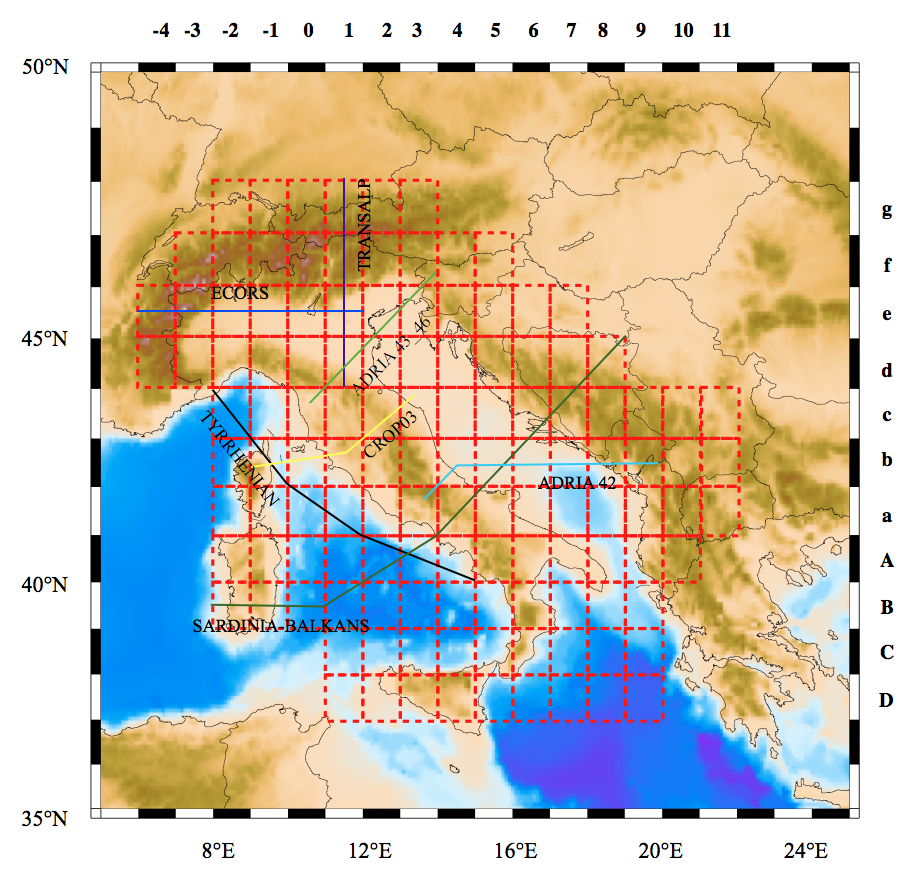
A detailed geodynamical interpretation for several profiles across the study area is elaborated using the obtained structural model. Some of these interpretations are developed starting from seismic reflection experiments profiles (e.g. CROP-ECORS and TRANSALP), others starting from geological sketches. The location of the sections is shown in Fig. 13. The aim of this effort is to enlighten and better understand the geodynamical setting in the Italic region, combining geophysical data (i.e. VS structural models) with geological interpretation and correlating them with heat flow and gravimetric data.
Figure 13. Interpreted sections.

Location of the interpreted sections presented in this paper, Figs. 14, 15, 16, 17, 20, 21, 22.
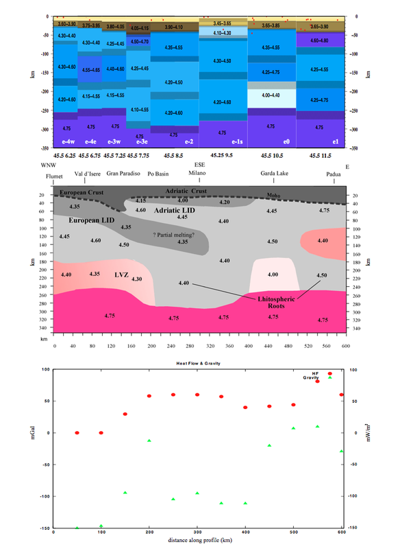
The section ECORS (Fig. 14), in the Western Alps, has been extended, to the east, to the Adriatic coast. This section allows to investigate the lithospheric-asthenospheric structure resulting from the European-Adriatic plates collisional process in the Western Alps, with a thick lid subducting eastward, marked by strong negative gravimetric anomalies. The presence of lithospheric roots is speculated in cells e-2 and e-1s (Milan), where an almost constant VS sequence extends to about 280 km of depth. In the same cells the VS of about 4.35 km/s between 90 km and 140 km depth likely indicates partial melting according to pyrolite phase diagram (Green and Ringwood, 1967). More to the east, just beneath the Moho, a 15-20 km thick mantle wedge is present (VS 4.00-4.20 km/s), possibly connected to the dehydration process of the downwelling slab. In cell e0 a LVZ (VS about 4.00 km/s) is clearly seen beneath the Garda zone at depth between 180 and 260 km, in accordance with the high heat flux and volcanism of the Eugani hills.
Figure 14. ECORS section.
Top: Cellular model of the drawn section along ECORS profile. Yellow to brown colors represent crustal layers, blue to violet colors indicate mantle layers. Red dots denote all seismic events collected by ISC with magnitude greater than 3 (1904-2006). For each layer VS variability range is reported. For the sake of clarity, in the uppermost crustal layers the values of VS are omitted. The error on thickness is represented by texture. All the values are reported in Appendix C.
Centre: Interpretation of the model (modified after Schmid and Kissling, 2000). The VS value reported may not necessarily fall in the centre of the VS range gained from inversion.
Bottom: Heat flow (mWm-2,red full circles) and gravimetric anomaly (mGal, green triangles) data along profile used to support our interpretation.
Figure 15. TRANSALP section.
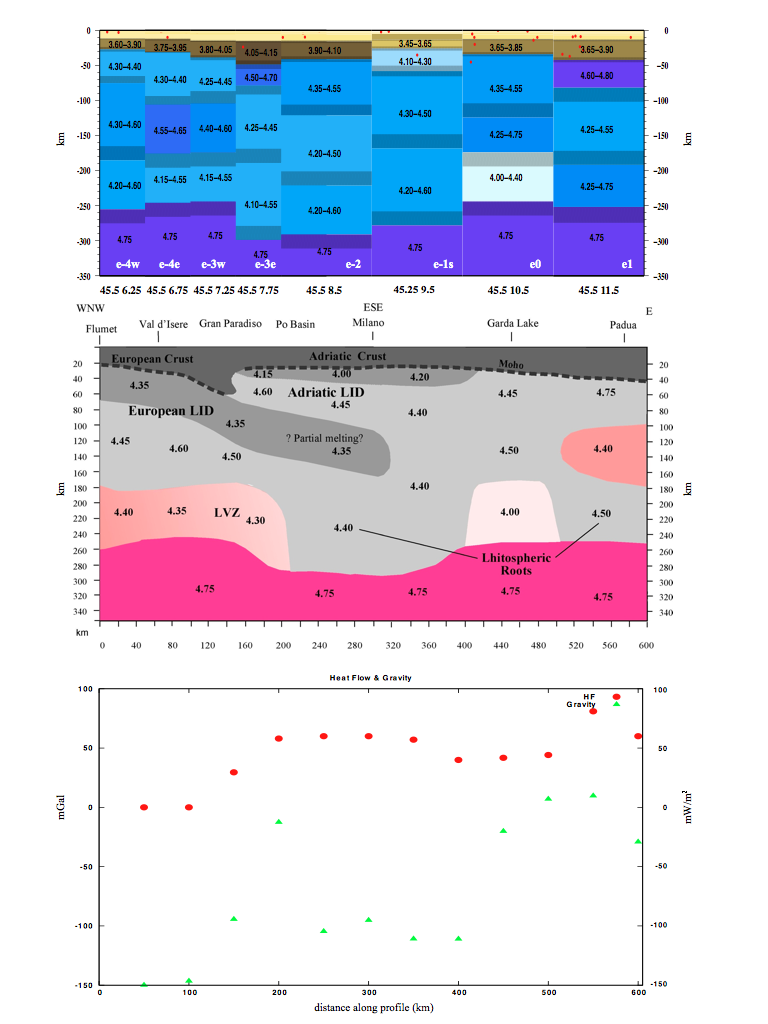
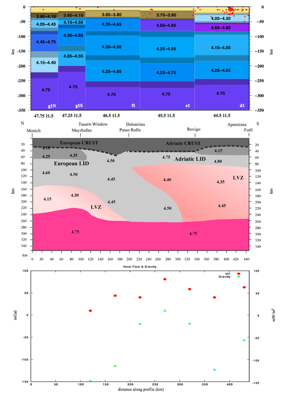
Top: Cellular model of the drawn section along TRANSALP profile. Yellow to brown colors represent crustal layers, blue to violet colors indicate mantle layers. Red dots denote all seismic events collected by ISC with magnitude greater than 3 (1904-2006). For each layer VS variability range is reported. For the sake of clarity, in the uppermost crustal layers the values of VS are omitted. The error on thickness is represented by texture. All the values are reported in Appendix C.
Centre: Interpretation of the model. The VS value reported may not necessarily fall in the centre of the VS range gained from inversion.
Bottom: Heat flow (mWm-2, red full circles) and gravimetric anomaly (mGal, green triangles) data along profile used to support our interpretation.
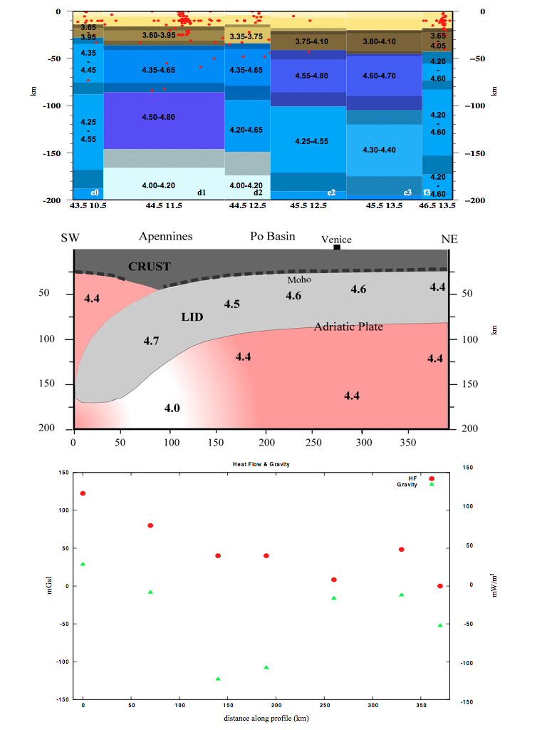
Figure 16. ADRIA 43_46 section.

Top: Cellular model of the drawn section across Northern Adriatic. Yellow to brown colors represent crustal layers, blue to violet colors indicate mantle layers. Red dots denote all seismic events collected by ISC with magnitude greater than 3 (1904-2006). For each layer VS variability range is reported. For the sake of clarity, in the uppermost crustal layers the values of VS are omitted. The error on thickness is represented by texture. All the values are reported in Appendix B.
Centre: Interpretation of the model, after a sketch of Cuffaro et al., 2009. The VS value reported may not necessarily fall in the centre of the VS range gained from inversion.
Bottom: Heat flow (mWm-2,red full circles) and gravimetric anomaly (mGal, green triangles) data along profile used to support our interpretation.
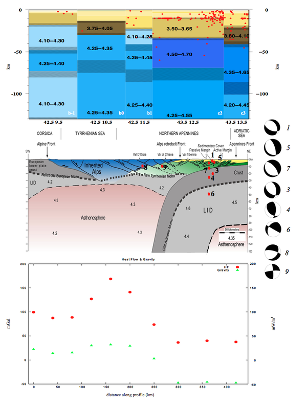
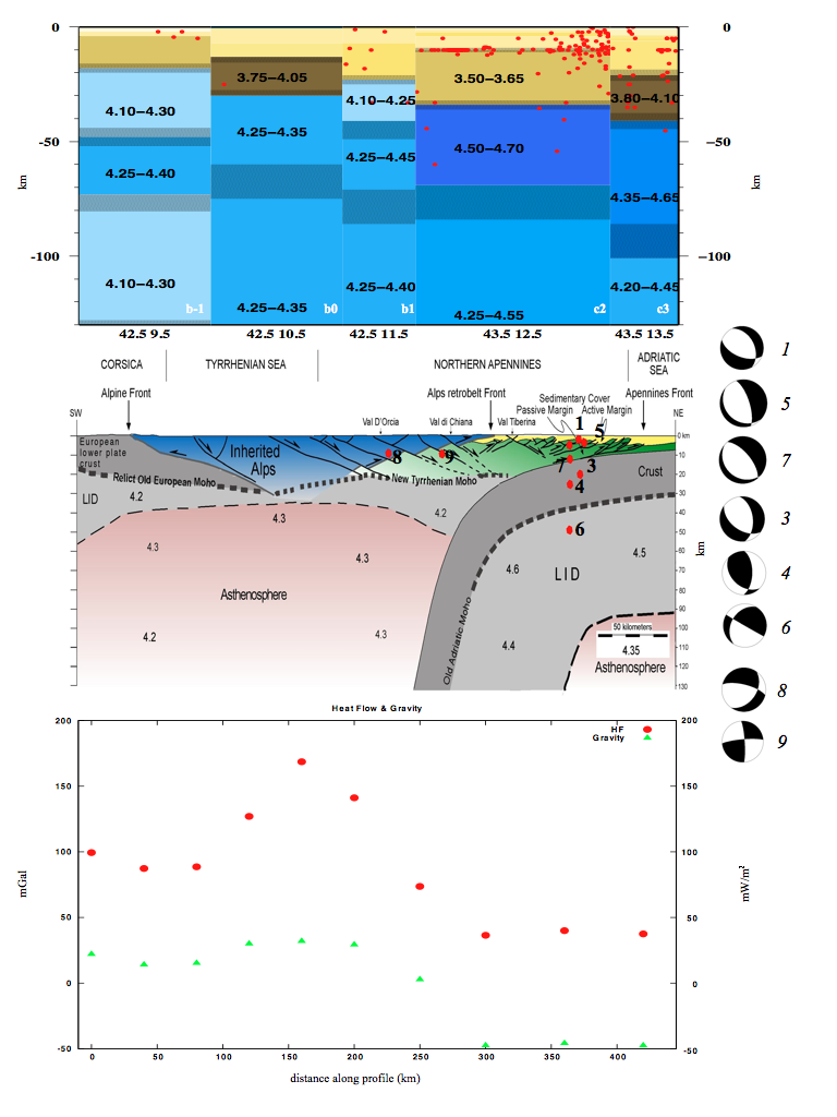
Figure 17. CROP03 section.
Top: Cellular model of the drawn section along CROP03 profile. Yellow to brown colors represent crustal layers, blue to violet colors indicate mantle layers. Red dots denote all seismic events collected by ISC with magnitude greater than 3 (1904-2006). For each layer VS variability range is reported. For the sake of clarity, in the uppermost crustal layers the values of VS are omitted. The error on thickness is represented by texture. All the values are reported in Appendix B.
Centre: Interpretation of the model, modified after Carminati and Scrocca (2004). The VS value reported may not necessarily fall in the centre of the VS range gained from inversion. The plotted hypocenters, and their focal mechanisms (on the right side), are retrieved by INPAR moment tensor inversion (see Appendix D for details).
Bottom: Heat flow (mWm-2,red full circles) and gravimetric anomaly (mGal, green triangles) data along profile used to support our interpretation.
The collisional process is clearly visible along the TRANSALP profile (Fig. 15), across the Central Alps. This section is extended to the Apennines in order to depict a complete cross-section of the Po Plain. Major elements highlighted are the subduction of the European lid beneath the Adriatic plate, well evidenced by a relatively fast VS-body dipping southward with significant crustal thickening beneath the Dolomites. The asthenospheric LVZ is well visible under both the European and Adriatic plates, in the former ranging between 150 km and 250 km of depth, in the latter from 90 km to 260 km. The negative gravity anomalies beneath Austro-Alpine (cells g1s and f1) and Apennines (cell d1) are well compatible with the presence of a sinking slab.
The Adriatic plate is also involved in two distinct tectonic processes: the south-westward or westward subduction beneath the Apennines and north-eastward subduction beneath the Dinarides.
The subduction beneath the Apennines (Fig. 16) is well modelled by the Adriatic Moho deepening and by a lid with VS about 4.50-4.70 km/s that reaches a depth of about 180 km beneath the north-eastern Apennines. A relatively fast asthenosphere extends beneath the Adriatic lithosphere, and the lower velocity (VS about 4.00 km/s) is reached above the sinking slab, likely witnessing of dehydration processes. Although in the northern Adriatic three distinct subduction zones coexist, (i.e. the Alpine, Apenninic and Dinaric) the Apenninic subduction seems to have a dominant role due to its present eastward migration, as marked by high seismicity and by the thickening toward NE of the Pliocene-Pleistocene sediments (Cuffaro et al., 2009).
The eastward migration of the Apenninic subduction likely causes loss of lithospheric material that should be replaced by uprising asthenospheric material (Doglioni et al., 1999). This is clearly evinced by the CROP03 profile (Fig. 17), where the Tyrrhenian asthenosphere rises up to 30 km depth, much shallower than the Adriatic asthenosphere, observed below about 90 km depth. The shallow Tyrrhenian asthenosphere feeds the Tuscan volcanism, as also marked by the high heat flow. On the contrary, very low heat flow and negative gravimetric anomalies characterize the subducting Adriatic lithosphere (cells c2 and c3) (Suhadolc et al., 1994), marked by a VS about 4.40-4.60 km/s and intermediate depth seismicity. In order to have a better understanding of the local stress field, and therefore of the geodynamic setting, the recent most damaging seismic events happened in the area (mostly Umbria-Marche seismic sequence of 1997), have been inverted with the INPAR method (Guidarelli and Panza, 2006) and superimposed on the section (Fig. 17). The detailed information about the moment tensor solutions for the events shown in Fig. 17 are given in Appendix D. Besides prevalent shallow normal faulting seismicity (Chimera et al., 2003), thrust-faulting intermediate depth seismicity is present in the subducting slab. An enlightening example of the improved resolving power of the INPAR method with respect to shallow, usually fixed, events, discussed in section “Methodology”, comes from the re-inversion of an event of the strong damaging Umbria-Marche seismic sequence in 1997 (event 4, Fig 17): the event, which occurred on October 6th, at 11:24:52 p.m. (43.06°N 12.80°E) is reported by CMT and RCMT bulletins as a normal-fault mechanism with depth fixed at 10 and 15 km, respectively. INPAR inversion determined a thrust-fault mechanism with a deeper focus, at depth of 27 km. (Fig. 18) To prove our argument we performed the inversion again, constraining the depth interval at 2-10 km and 2-16 km respectively: as we could expect, the former inversion gives a normal fault mechanism at 2 km depth, while the latter gives a thrust fault mechanism at 16 km depth, therefore at the deepest limit of our fixed interval, suggesting to search for a deeper focus (Fig. 19).
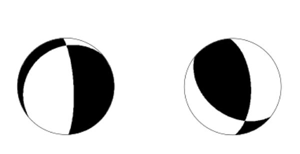
Figure 18. CMT vs INPAR focal mechanisms.

The focal mechanism for the event of October 6th, 1997 at 11:24:52 p.m. (43.06°N 12.80°E), Umbria-Marche sequence, as retrieved by CMT (nodal planes: 149 23 -73/310 68 -97) (left) and INPAR (nodal planes: 135 41 52/1 59 118) (right). The focal depth, fixed by CMT, is 10 and 27 km, respectively. The different resolving power of the two inversion methods determines an opposite focal mechanism, normal-faulting the former, thrust faulting the latter.
Figure 19. INPAR vs depth focal mechanisms.
The same event of Figure 18 inverted with the INPAR method constraining depth at two different intervals: 2-10 km (nodal planes: 229 21 -40/357 77 -106) (left) and 2-16 km (nodal planes: 128 42 50/357 59 120) (right). The retrieved depth is 2 km and 16 km, respectively. The focal mechanism is opposite: normal the former (left), thrust the latter (right). The wrong fault-plane solution is determined constraining the event at shallow depth (see Appendix D for details).
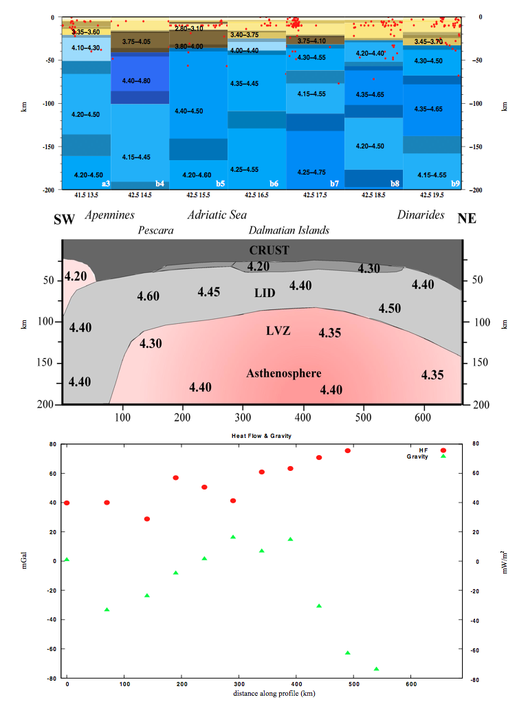
The two opposing-side subduction processes of the Adriatic plate under the Apennines and Dinarides are clearly distinguishable in Fig. 20, which is a cross section of the Adriatic at about 42°N latitude. The westward Apenninic subduction is highlighted by relatively fast (VS 4.40-4.60 km/s) lithosphere dipping to the west, marked by relatively low heat flow and negative gravity anomaly. A mantle wedge (VS about 4.20 km/s) is likely to be present at the top of the subducting lithosphere, in the upper plate, as a result of both dehydration and mantle compensation. To the east, the lithosphere gets thinner, with partial melt likely to be present offshore Adriatic at about 50 km depth (VS 4.20 km/s), with relatively high heat flow and positive gravity anomaly possibly associated to rifting process. To the east of the Dalmatian islands, the lithosphere gets gradually thicker, due to the north-eastward directed subduction with a lower dip angle compared to the Apennines subduction. According to Cuffaro et al. (2009), the Dinarides are older than the Appenines, but they were downward tilted by the eastward migration of the Apennines subduction hinge and the thrust-belt front, after being sub-aerially eroded, has been subsided.
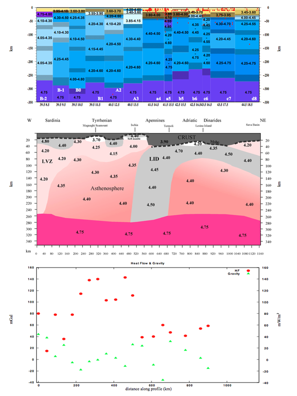
The same process can be seen in Fig. 21, that is, a SW-NE trending profile from Tyrrhenian to the Sava Basin. The westward subducting Apenninic lithosphere is almost vertically bent by the mantle easterly directed flow, while the Dinaric eastward subduction has a dip angle of about 20-30°, as discussed in detail by Doglioni et al. (1999) and Carminati et al. (2004). A mantle wedge is visible in both upper plates of the Dinaric and Apenninic subductions by low velocities layers (VS 4.00 km/s and 4.20 km/s). To the west, the eastward retreat of the Apenninic subduction calls for a mantle compensation represented by the uprising LVZ beneath the Tyrrhenian Sea. This shallow asthenospheric material directly feeds Tyrrhenian volcanoes as Magnaghi and Ischia, as fairly supported by heat flow peaks.
It is well known that the Tyrrhenian Sea started opening about 15 Ma, as the result of the backarc expansion (Scandone, 1980; Gueguen et al., 1997 and reference therein) process induced by the eastward migration of the Apenninic subduction (Royden and Burchfield, 1989; Doglioni, 1991), which took place in the late Oligocene on the preexisting alpine-betic orogen. The Tyrrhenian Sea is still opening, with age of the newly formed oceanic lithosphere decreasing from west to east. This process was likely inhomogeneous and asymmetric. Clear evidence of this are the numerous “boudins” disseminated in the basin at different scales. A “boudin” is a continental isolated block, common at the mesoscale, as the product of extension of a competent layer (i.e. with high resistance to deformation and loss of thickness) within a less competent matrix (Ramsay and Huber, 1983, and references therein). The “boudins” are bounded by thinned areas (necks) where material with lower viscosity flows.
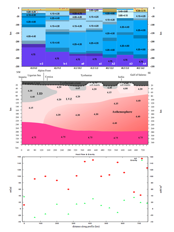
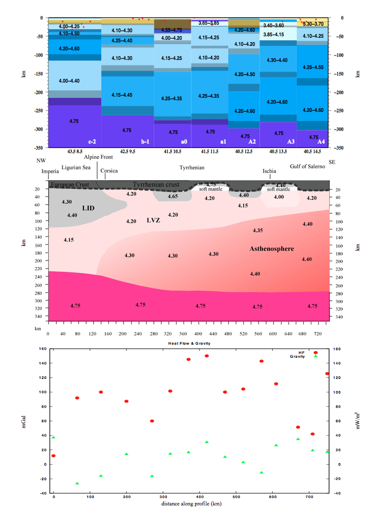
The distance between “boudins” is in the order of the original lithospheric thickness, ranging from 100 to 400 km as argued in Gueguen et al. (1997). The most prominent one is the Sardinia-Corsica block (Fig. 21, cells a-2, A-1, B-1), where the lithosphere preserves its original thickness (about 70 km), which represents a fragment of the Betic foreland. To the east a thin neck extends with a lithospheric thickness of about 25-30 km (Magnaghi basin) down to cell A2, where an intra-Tyrrhenian “boudin” is located, likely representing a fragment of the hinterland of the previous Alpine-Betic orogen. Generally crustal thickness reflects the lithospheric thickness, being about 20-25 km beneath “boudins”, and 10-15 km and even less beneath necks. Another intra-Tyrrhenian “boudin” is located in cell a0 (see Figure 22), with a thin neck that separates it from cell A2.
Figure 20. ADRIA 42 section.

Top: Cellular model of the drawn section across central Adriatic. Yellow to brown colors represent crustal layers, blue to violet colors indicate mantle layers. Red dots denote all seismic events collected by ISC with magnitude greater than 3 (1904-2006). For each layer VS variability range is reported. For the sake of clarity, in the uppermost crustal layers the values of VS are omitted. The error on thickness is represented by texture. All the values are reported in Appendix B.
Centre: Interpretation of the model, after a sketch of Cuffaro et al., 2009. The VS value reported may not necessarily fall in the centre of the VS range gained from inversion.
Bottom: Heat flow (mWm-2,red full circles) and gravimetric anomaly (mGal, green triangles) data along profile used to support our interpretation.
Figure 21. SARDINIA-BALKANS section.
Top: Cellular model of the drawn section from Sardinia to Balkans. Yellow to brown colors represent crustal layers, blue to violet colors indicate mantle layers. Red dots denote all seismic events collected by ISC with magnitude greater than 3 (1904-2006). For each layer VS variability range is reported. For the sake of clarity, in the uppermost crustal layers the values of VS are omitted. The error on thickness is represented by texture. All the values are reported in Appendix B.
Centre: Interpretation of the model. The VS value reported may not necessarily fall in the centre of the VS range gained from inversion.
Bottom: Heat flow (mWm-2,red full circles) and gravimetric anomaly (mGal, green triangles) data along profile used to support our interpretation.
Figure 22. Tyrrhenian section.
Top: Cellular model of the drawn section across Tyrrhenian. Yellow to brown colors represent crustal layers, blue to violet colors indicate mantle layers. Red dots denote all seismic events collected by ISC with magnitude greater than 3 (1904-2006). For each layer VS variability range is reported. For the sake of clarity, in the uppermost crustal layers the values of VS are omitted. The error on thickness is represented by texture. All the values are reported in Appendix B.
Centre: Interpretation of the model. The VS value reported may not necessarily fall in the centre of the VS range gained from inversion.
Bottom: Heat flow (mWm-2, red full circles) and gravimetric anomaly (mGal, green triangles) data along profile used to support our interpretation.
Below, along the NE-SW direction of the Tyrrhenian expansion, a rising LVZ is present, likely representing the eastward mantle flow gradually emerging in the hanging wall of the Apennines retreating slab.
Heat flow and gravimetric data substantially support this picture, with the highest peak of heat flow below Magnaghi, Ischia and cell a1, likely feeding the Alban Hills, and evident gravimetric negative anomalies corresponding to the “boudins”.